Evidence for Crustal Motion

Additional evidence was needed to support the idea of seafloor spreading. As oceanographers, geologists, and geophysicists explored the Earth’s crust on land and under the oceans, evidence began to accumulate.

Epicenters of earthquakes were known to be distributed around the Earth in narrow and distinct zones. Epicenters are the points on the Earth’s surface directly above the earthquake location. These zones were found to correspond to the areas along the ridges, or spreading centers, and the trenches, or subduction zones. Earthquakes that occur between the crust’s surface and 100 km (60 mi) in depth are known as shallow quakes.

These are prevalent along ridges and rises and at trenches where the lithosphere is fractured. Earthquakes occurring at depths greater than 100 km (60 mi) below the crust are called deep quakes. They occur in subduction zones, and the deeper the earthquakes are the more they are displaced landward, beneath continents and island arcs (fig. 2.9).

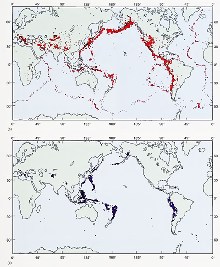
Fig. 2.9. Earthquake epicenters, 1961-67. (a) Epicenters of earthquakes with depths less than 100 kilometers outline regions of crustal movement, (b) Epicenters of earthquakes with depths greater than 100 kilometers are related to subduction

Researchers sank probes into the sea floor to measure the heat from the interior of the Earth moving through the crust (fig. 2.10). The measured heat flow shows a pattern with a high degree of variability, even over closely spaced intervals. In part, this variation in the data is attributed to the seeping of seawater down through porous or fractured portions of the crust at one location along a ridge system and its rising as heated water at another.

Fig. 2.10. Preparing to lower a heat flow probe. The probe consists of a cylinder holding the measuring and recording instruments above a thin probe that penetrates the sediment. Thermisters (devices that measure temperature electronically) at the top and bottom of the probe measure the temperature difference over a fixed distance equal to the length of the probe. This temperature change with depth is used to compute the heat flow through the sediment

This circulation does not occur over regions of the sea floor that are sealed by a thick layer of loose particles, or sediment. In these areas, the measured heat flow shows a regular pattern. It is highest in the vicinity of the mid Ocean ridges over the ascending portion of the mantle convection cell where the crust is more recent, and it decreases as the distance from the ridge center and the crustal age increases (fig. 2.11).

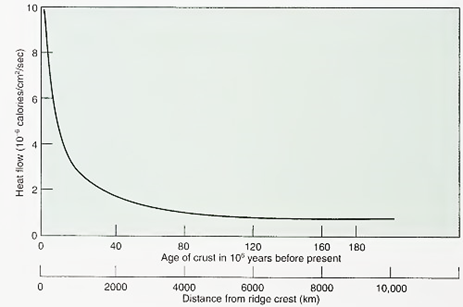
Fig. 2.11. Heat flow through the Pacific Ocean floor. Values are shown against age of crust and distance from the ridge crest. Data from], G. Sclater andJ. Croive, On the Variability of Oceanic Heat Flow Average in Journal of Geographical Research, 81:17 (June 1976), p, 3004. American Geophysical Union, Washington, D.C.

Radiometric dating of the age of rocks from the land and from the sea floor shows that the oldest rocks from the oceanic crust are only about 200 million years old, whereas the rocks from the land are much older. The sea floor formed by convection-cell processes at the spreading centers is young and short-lived, for it is lost at the subduction zones, where it plunges back down into the mantle.

Vertical, cylindric samples, or cores, were obtained by drilling through the sediments that cover the ocean bottom and into the rock of the ocean floor. (A detailed discussion of sediment is found in chapter 3.) Drilling cores through the average of 500-600 m (1600-2000 ft) of sediments that cover the deep-ocean floor and then drilling on into the ocean floor required the development of a new technology and a new kind of ship.

In the late summer of 1968 the specially constructed drilling ship Glomar Challenger (see prologue fig. XIX) was used for a series of studies. This ship, 122 m (400 ft) long, with a beam of 20 m (65 ft) and a draft of 8 m (27 ft), displaces 10,500 tons when loaded. Its specialized bow and stern thrusters and its propulsion system respond automatically to computer-controlled navigation, using acoustic beacons on the sea floor.

This setup enables the ship to remain for long periods of time in a nearly fixed position over a drill site in water too deep to anchor. An acoustic guidance system enables it to replace drill bits and reenter the same bore holes in water about 6000 m (20,000 ft) deep. This method is illustrated in figure 2.12. A more general discussion of cores and coring methods is found in chapter 3.

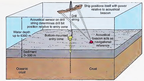
Fig. 2.12. Deep-ocean drilling technique. Acoustical guidance systems are used to maneuver the drilling ship over the bore hole and to guide the drill string back into the bore hole

In 1983 the Glomar Challenger was retired, after logging 600,000 km (375,000 mi), drilling 1092 holes at 624 drill sites, and recovering a total of 96 km (60 mi) of deep-sea cores for study. A new deep-sea drilling program with a new drill vessel, the JOIDES Resolution, began in 1985. The JOIDES Resolution is about the same size as the Glomar Challenger, complete with the world’s most sophisticated, state-of-the-art scientific and drilling equipment (fig. 2.13). Information on the current research being conducted by the JOIDES Resolution will be found in section 2.7.

The cores taken by the Glomar Challenger provided much of the factual data needed to establish the existence of seafloor spreading. No ocean crust older than 180 million years was found, and sediment age and thickness were shown to increase with distance from the ocean ridge system (fig. 2.14). Note that the sediments closest to the ridge system are thin over the new crust that has not had long to accumulate its sediment load. The crust farther away from the ridge system is older and is more heavily loaded with sediments.

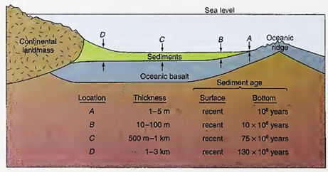
Fig. 2.14. Age and thickness of seafloor sediments

Although each of these pieces of evidence fits the theory that the Earth’s crust produced at the ridge system is new and young, the most elegant proof for seafloor spreading came from a study of the magnetic evidence locked into the oceans’ floors.

The Earth’s familiar north and south geographic poles at 90°N and 90°S latitude mark the axis about which it rotates. The Earth also behaves as if it had a giant bar magnet embedded in its interior tilted 11° away from the axis of rotation. The magnetic North Pole is located in the Hudson Bay area, and the magnetic South Pole is directly opposite in the South Pacific Ocean. Like any magnet, the Earth is surrounded by a magnetic field.

Its lines of force converge and dip toward the Earth at the magnetic poles and are parallel to the Earth at the magnetic equator. At other positions on the Earth’s surface, the lines of force have both horizontal and vertical components (fig. 2.15). A magnetic field like the Earth’s, with two opposite poles, is called a dipole.

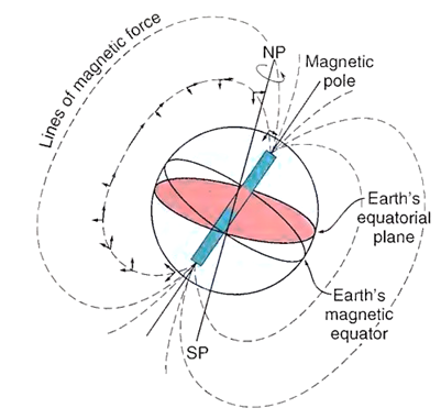
Fig. 2.15. Lines of magnetic force surround the Earth and converge at the magnetic poles. The lines of force have components that are parallel and perpendicular to the Earth’s surface. The vertical components are not present at the Earth’s magnetic equator and arc at their maximum at the magnetic poles, where the horizontal components disappear. A compass orients its needle with the horizontal component to indicate the direction to the magnetic pole. NP and SP indicate the present north and south geographic poles

When materials that can be magnetized are heated in a magnetic field they become magnetized as they cool, with their north and south magnetic poles lined up with the poles of the magnetic field. In the same way, when molten volcanic material cools and solidifies, its iron-bearing minerals become magnetized and permanently aligned with both the horizontal and vertical components of the Earth’s magnetic field.

Research on age-dated layers of volcanic rock found on land shows that the polarity, or north-south orientation, of the Earth’s magnetic field reverses for varying periods of geologic time. Thus, at different times in the Earth’s history the present north and south magnetic poles have changed places. Each time a layer of volcanic material cooled and solidified, it trapped the magnetic orientation and polarity of the time period in which it occurred. The dating and testing of samples taken through a series of volcanic layers have enabled scientists to build a calendar of these events (fig. 2.16).

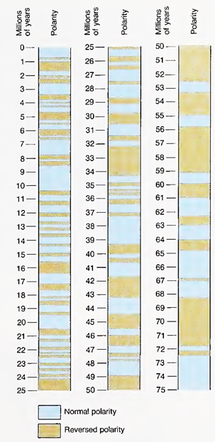
Fig. 2.16. Polarity reversal time scale during the Cenozoic Era. Time is given in millions of years

During these polar reversals, the Earth’s magnetic field gradually decreases in strength by a factor of about 10 over a period of a few thousand years. There is some evidence that during a reversal the Earth’s field may not remain a simple dipole. The collapse of the magnetic field during reversals enables more-intense cosmic radiation to penetrate the planet’s surface, and recent work has suggested a correlation between such periods and a decrease in populations of delicate, single-celled organisms that live in the surface layers of the ocean.

Nearly 170 reversals have been identified during the last 76 million years, and the present magnetic orientation has existed for 780,000 years. The interval between reversals has varied, with some notable periods of constant orientation for long time intervals. During the Cretaceous Period (from roughly 120 million to 80 million years before present) the field was stable and normally polarized. The field was stable and reversely polarized for about 50 million years in the Permian Period, roughly 300 million years before present. The cause of reversals is unknown but is thought to be associated with changes in the motion of the magnetic material of the Earth’s liquid outer core. How long our current polarity will last we do not know.

When magnetometers were towed over the sea floor by scientists from the Scripps Institution of Oceanography in the early 1960s, the resulting maps revealed a mirror-image pattern of parallel magnetic stripes on each side of the mid-ocean ridge (fig. 2.17).

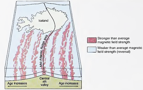
Fig. 2.17. Reversals in the Earth’s magnetic polarity cause the symmetrically striped pattern centered on the Mid-Atlantic Ridge. The age of the sea floor increases with the distance from the ridge. The spreading rate along the Mid-Atlantic Ridge is about one centimeter per year

Their significance was not understood until 1963, when F. J. Vine and D. H. Matthews of Cambridge University proposed that these stripes represented a recording of the polar reversals of the vertical component of the Earth’s magnetic field, frozen into the sea floor; As the molten basalt rose along the crack of the ridge system and solidified, it locked in the direction of the prevailing magnetic field. Seafloor spreading moved this material off on either side of the ridge, to be replaced by more molten materials. Each time the Earth’s magnetic field reversed, the direction of the magnetic field was recorded in the new crust.

Vine and Matthews proposed that if such were the case, there should be a symmetric pattern of magnetic stripes centered at the ridges and becoming older away from the ridges. Their ideas were confirmed; the polarity and age of these stripes corresponded to the same magnetic field changes found in the dated layers on land and dramatically demonstrated seafloor spreading.

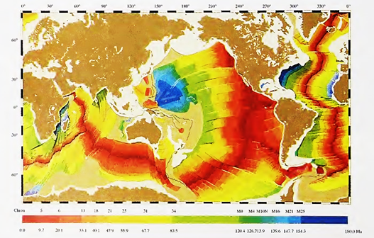
Fig. 2.18. The age of the ocean floor is shown in this color-shaded relief image based on sea-floor spreading magnetic anomalies. Blue regions represent ocean floor created during the Mesozoic Era (more than 140 Ma); red indicates young ocean floor near the mid-ocean ridges. Oceanic fracture zones, which offset the spreading centers, are highlighted by artificial illumination. This image was produced from a digital age grid with a 10-kilometer grid interval. Ma (or megannums) = millions of years ago. Chrons identify boundaries of magnetic polarity states, normal or reversed

The accumulation of magnetic stripe data across the world’s oceans has been used to produce a map of the age of the sea floor (fig. 2.18). Seafloor age increases away from the oceanic spreading centers, providing another verification of seafloor spreading. The present ocean basins are not old but new, created during the past 200 million years, or the last 5% of the Earth’s history.