Mathematical Desctiption of Environmental Models

The environmental models are normally described by systems of partial differential equations (PDEs). The number of equations is equal to the number of chemical species studied by the modes and the unknown functions are concentrations ofthese species. Five basic stages are described in the development of a large environmental model:

- one has to select the physical and chemical processes that are to be taken into account during the development of the model,
- the selected processes must be described mathematically,
- the resulting system of PDEs must be treated by numerical methods,
- the reliability of the obtained results must be evaluated and
- conclusions should be drawn.

It is important to take into account all relevant physical and chemical processes during the development of the models. If more physical and chemical processes are included in the model, then one should expect that more accurate and more reliable results can be calculated. However, two difficulties are related to the attempt to include as many as possible physical and chemical processes in the model:

- The complexity of the model is increased when more processes are included in it. The treatment of the model on the available computers might become very difficult, and even impossible, when too many processes are taken into account.

- Some physical and chemical processes are still not well understood, which means that such processes must either be neglected or some simplified mechanisms, based on uncertain assumptions and/or on experimental data, must be developed.

It is necessary to find a reasonable compromise related to the number of processes that are to be taken into account when a large environmental model is developed. This reasoning explains also why it is necessary to validate the model results.

The selected physical and chemical processes have to be described by mathematical terms. Some more- or less-standard rules exist that can be used for the mathematical description of different processes. Several examples, which are related to air pollution modes, are listed below:

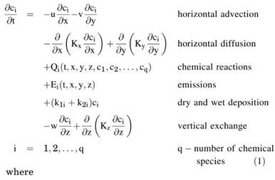
- The transport caused by the wind (called advection) is described by using terms that contain first-order spatial derivatives of the unknown functions (the concentrations of the studied pollutants) multiplied by the wind velocities.

- The diffusion of the concentrations is expressed by second-order spatial derivatives multiplied by the diffusivity coefficients.

- The chemical reactions are represented by nonlinear mathematical terms.
- The change of the concentrations in time is given by first-order derivatives of the concentrations of the pollutants with respect to time.

It should be stressed here that the above rules are applicable not only to air pollution models but also to many other environmental models.

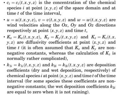
When all selected physical and chemical processes are expressed by some mathematical terms, then these terms have to be combined in a system of PDEs. For example, when long-range transport air pollution is studied, the system of PDEs, which represents the mathematical model, can be written as follows (it should be mentioned that similar systems are used in other environmental models):

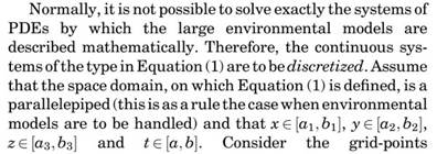
It is assumed here that Cartesian coordinates have been chosen. Other coordinates, for example, spherical coordinates, can also be used.

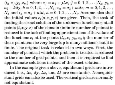
The above two remarks illustrate the fact that the discretization can be performed in different ways. The important thing is that the main idea remains the same: One considers approximate values of the unknown functions at a finite number of grid-points, which are defined by the discretization chosen, instead of the exact solution of Equation (1) on the whole continuous space domain.

Numerical methods must be used to find approximate values of the solution at the grid-points. It is also appropriate to split the model, the system of PDEs of the type in Equation (1), into several submodels (subsystems), which are in some sense simpler. Another advantage when some splitting procedure is applied is that the different subsystems have different properties, and one can try to select the best numerical method for each subsystem.

It is clear that if some splitting procedure and appropriate numerical methods are already chosen, then any continuous system of the type in Equation (1), which represents an environmental model, is replaced by several discrete submodels that have to be treated on the available computers.

As mentioned above, the model described by Equation (1) is an air pollution model. However, it must be emphasized, once again, that many environmental models are also described by systems of partial differential equations and, thus, can be treated similarly.