Response Functions to Interacting Drivers. Self-Thinning

Each process has a typical response function to its major driver—for example, net assimilation to light, or respiration to temperature. These response functions can be linear (Fig. 13.1) but also curvilinear or even exponential. However, typically, processes are driven by multiple factors. In this case, nonlinear and irregular behaviour might set in. One example of such interacting drivers is the response of soil respiration to soil temperature and soil water availability. As long as soil moisture is abundant, soil respiration increases exponentially with temperature (Lloyd and Taylor 1994).

However, as soon as soil water availability becomes limiting, soil respiration rates are much lower than those modelled by an exponential temperature response function (Ruehr et al. 2010; Fig. 13.2). Often one can determine threshold values below which soil water availability becomes the dominant driver. However, such thresholds are generally site specific; that is, they depend on soil and vegetation characteristics, and vary temporally—for example, with the time of the year and thus vegetation phenology.

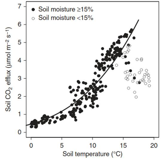
Fig. 13.2. The dependence of sod respiration (daily averages) in a mixed temperate forest on soil temperature differs depending on soil water availability. Data are given for 2006. The Lloyd and Taylor model (R² = 0.83) is given only if soil moisture ≥15%, depicted with filled symbols. Open symbols stand for soil moisture <15%. Soil respiration (SR) = 2.58 e^{419.6(1/56.02)-1/(T-46.02)}. (Data from N. Ruehr)

Self-Thinning. Some processes, such as the production of plant biomass in a stand, are driven not only by interacting environmental drivers but also by density-dependent effects. For example, intra- and interspecies competition, but also the occurrence and severity of pathogen and parasite damage affect a stand’s productivity. Self-thinning occurs when plants in dense plant populations or communities compete vigorously with each other for resources and some die, in turn decreasing the density of the survivors. The increasing growth rate of the survivors leads to continuous competition, increasing mortality, thus decreasing the number of survivors even further. Yoda et al. (1963) formalised this relationship and expressed the biomass of individual plants (W) as a function of the density of individual plants (n) in a stand, where c is a proportionality factor depending on light and nutrient supply:

This equation states that the biomass of an individual plant declines when plant density in this stand is increasing. Since this relationship holds for many different plant communities (Fig. 13.3), this relationship is also called the -3/2 power law, with -3/2 being the selfthinning constant. This constant can be explained by the spatial expansion of the biomass (threedimensional volume, exponent 3) and the expansion of this biomass per unit of ground (two-dimensional area, exponent 2; Osawa and Allen 1993).

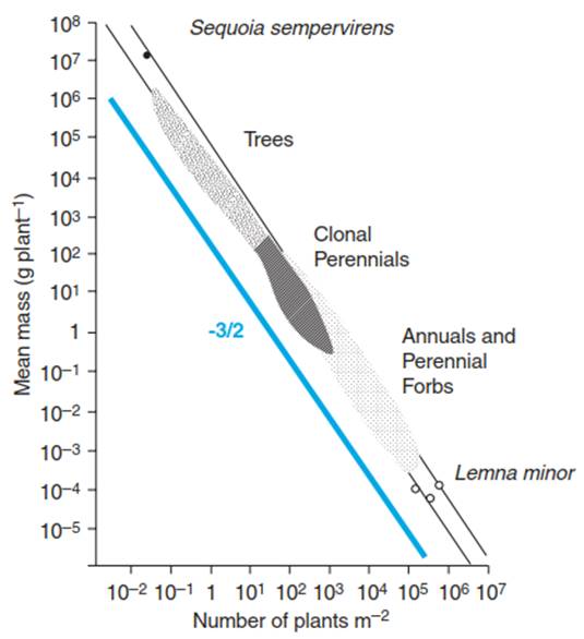
Fig. 13.3. Self-thinning in different communities. When the logarithm of the average plant weight is plotted as a function of the logarithm of the stand density, the data generate a line with a slope of -3,2. (After Silvertown and Lovett Doust (1993))

Expressing this self-thinning law based on plant biomass per ground area (B), thus multiplying the individual plant biomass (W) with the number of plants per unit of ground (n), results in:

Taking the logarithm of this equation yields the linear equation:

This equation shows that the maximum biomass of a monospecific stand that can be achieved in an area depends on the number of individual plants. The slope (-1/2) applies to a broad range of growth forms (herbaceous plants, shrubs, trees) (Westoby 1984), while the parameter c describes the productivity, which is determined by many factors such as the site conditions and growth characteristics of the species.

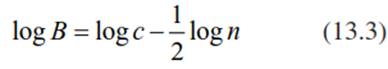
Thus, in a managed forest stand, density- dependent effects mean that after an exponential growth phase up to canopy closure, a phase of self-thinning follows, during which mortality occurs. The growth rate of the stand decreases (in comparison with the exponential growth rate in the early stages) and the standing biomass reaches a certain level (Fig. 13.4a). The maximum attainable biomass then depends on the climate, vegetation structure, nutrient supply and management, as a result of plant plasticity to increased competition and of mortality. Climate conditions lead to regional differentiation—for example, the yield of forests in southern Germany is higher than that in northern Germany because of higher annual irradiance in the south.

Fig. 13.4. Relationships between standing biomass and stand age. a Increase in biomass with age of trees in managed spruce forests in Germany compared with unmanaged forests of spruce, pine and larch in eastern Europe and Siberia (Schulze et al. 1999). It is shown that even unmanaged forests reach maximum biomass. This is not the result of an equilibrium between assimilation and respiration; it is the result of different stress impacts (fire, wind). b Influence of forest management—that is, thinning—on the development of a spruce stand in southern Sweden. The zig-zag path in the development of the stand is due to the removal of biomass in forest management and the subsequent recovery of the stand. (After Kramer (1988))

In managed systems, the biomass (and thus the competition among trees) is additionally controlled by different management practices such as thinning in forestry (Fig. 13.4b). Overall, the development over time of many processes resembles a saturation function (Schulze 1982), both for forests and for agricultural systems. However, in some systems—for example, intensively managed grasslands—the saturation plateau is rarely reached because mowing of such grasslands typically takes place during the exponential growth phase, when forage quality is very high, well before the biomass reaches the saturation plateau. Thus, the managed grassland is permanently kept at a juvenile stage, when regeneration growth of new foliage replaces the cut biomass.