Stomatal Responses to Environmental Factors

Carbon dioxide: Stomata react to the gradient in the CO₂ concentration between the external air and the intercellular spaces of the leaves. In a classical experiment, Raschke (1972, 1979) was able to open stomata by decreasing the CO₂ concentration down to a CO₂-free environment and close them by increasing the CO₂ concentration until saturation was reached. Neither light nor darkness influenced the observed CO₂ concentration effects. The CO₂ gradient between the leaf and the air, as expressed by the CO₂ concentration ratio, C_i/C_a, remains the main variable to model photosynthesis.

Epidermal water status: With decreasing turgor in the epidermis, the aperture of the stomata decreases (Nonami et al. 1990). In contrast to the reaction of the leaf to changes in the root water potential, this is a cellular imbalance in the epidermal turgor dependent on transpiration (Schulze 1993).

Light: Stomata open with increasing light intensity. In the morning, stomatal conductance increases earlier than photosynthesis. Therefore, stomata do not limit the uptake of CO₂ during the early morning when the humidity is high.

Temperature: At low temperatures (freezing point), stomata are closed, and they open as the temperature increases. This opening is exponential at temperatures above 40 °C, so the leaf temperature can decrease even below that of the air because of the strong cooling by transpiration if water is available and under low rH values.

Air humidity and leaf water status: Stomata close with an increasing vapour pressure deficit between the leaf and the air, and this can also be observed with an isolated epidermis (Lange et al. 1971), where closing is faster than opening (Fig. 10.22a). This response can be so strong that transpiration decreases despite an increasing water vapour gradient between the leaf and the air (Fig. 10.22b; Schulze et al. 1972). It is still unclear how stomata “measure” humidity. From measurements with He-enriched air, Peak and Mott (2011) proposed that water vapour is the driving force for the stomatal response to humidity.

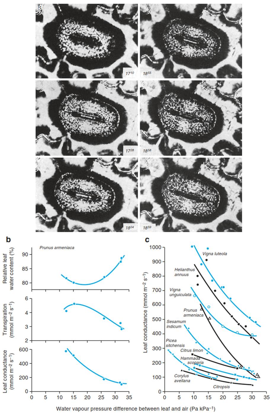
Fig. 10.22. Stomatal response to air humidity. a Stomata in isolated epidermis of Polypodium vulgare. The lower surface of the epidermis was in contact with water. Only a small air bubble simulated the sub-stomatal air space. On the upper surface, dry or moist air was blown over the stomata with a capillary. The experiment started with closed stomata in dry air. A change to moist air induced slow stomatal opening within 54 min. With constant moist conditions the stomata stayed open, but upon application of dry air they closed within 4 min (Lange et al. 1971). b Response of measured leaf conductance, transpiration and water content of a Prunus armeniaca leaf to dry air. The stomata closed, transpiration decreased and leaf water content increased (Modified from Schulze et al. (1972)). c Responses of different types of plant to dry air. (Schulze and Hall 1982)

In tall trees the reaction to local deficits probably plays an important role in the regulation of stomata during the course of the day. In the canopy of a forest, turbulence of air movement occurs with fast exchanges of air packages with differing humidity. This correlates with fast changes in xylem flow. Neighbouring trees exposed to the same air masses show synchronous changes in xylem flow (Hollinger et al. 1994). Stomatal closure is induced by short-term changes in transpiration and the associated changes in the water state of the epidermis (Kostner et al. 1992). As closure is faster in dry air than opening is in moist air, a continuous decrease in stomatal conductance during the day is the consequence of fluctuating humidity in the atmosphere.

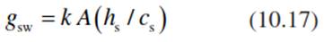
The stomatal response to humidity has been presumed to be a function of the driving force of transpiration, D_L, the gradient of water vapour concentration between the leaf and the air (Eq. 10.15), even though the response to D_L decreases with temperature. Also, with stomatal conductance as defined by D_L, no common relation with CO₂ assimilation can be observed. However, if the response of stomatal conductance to water vapour, g_sw (measured in moles per square metre per second), is scaled to relative humidity at the leaf surface (h_s) and to the mole fraction of CO₂ at the leaf surface (c_s), a linear relation emerges. This includes the response to CO₂ assimilation, A, and to air humidity at different temperatures, with к being an empirical coefficient, 9.31, which may depend on the species (Ball et al. 1987).

Equation 10.17 is interesting in view of the biophysics of stomatal regulation, because the relative humidity at the leaf surface would express the water potential at the site of evaporation (see Eq. 10.7), and it would be an expression of the “hydration of the evaporating surfaces in the mesophyll”, which could regulate stomata. Pieruschka et al. (2010) suggest that the driving force for all stomatal responses to the environment is radiation, which controls the water vapour production in the leaf interior.

References:
Aloni R (2004) The induction of vascular tissues by auxin. In: Davies PJ (ed) Plant hormones. Kluwer Academic Publisher, Dortrecht

Ball JT, Woodrow IE, Berry JA (1987) A model predicting stomatal conductance and its contribution to the control of photosynthesis under different environmental conditions. Progr Photosynth Res 4:221-224

Bohm J (1893) Capillaritat und Saftsteigen. Ber Dtsch bot Ges 11:203-212
Bonner J, Galson AW (1952) Principles of plant physiology. Freeman, San Francisco
Bryukhanova M, Fonti P (2013) Xylem plasticity allows rapid hydraulic adjustment to annual climatic variability. Trees 27:485-496

Burgess SSO, Adams MA, Turner NC, White DA, Ong CK (2001) Tree roots: conduits for deep recharge of soil water. Oecologia 126:158-165
Burkhardt J (2010) Hygroscopic particles on leaves: nutrients or desiccants? Ecol Monogr 80:369-399

Canadell J, Jackson RB, Ehleringer JR, Mooney HA, Sala OE, Schulze E-D (1996) Maximum rooting depth of vegetation types at the global scale. Oecologia 108:583-595

Carlquist S (1991) Anatomy of vine and liana stems: a review and synthesis. In: Putz FE, Mooney HA (eds) The biology of vines. Cambridge University Press, Cambridge

Choat B, Jansen S, Brodribb TJ, Cochard H, Delzon S, Bhaskar R, Bucci SJ, Feild TS, Gleason SM, Hacke UG, Jacobsen AL, Lens F, Maherali H, Martinez- Vilalta J, Mayr S, Mencuccini M, Mitchell PJ, Nardini A, Pittermann J, Pratt RB, Sperry JS, Westoby M, Wright IJ, Zanne AE (2012) Global convergence in the vulnerability of forests to drought. Nature 491:752-755

Cirelli D, Jagels R, Tyree MT (2008) Towards an improved model of maple sap exudation: the location and role of osmotic barriers in sugar maple, butternut, and white birch. Tree Physiol 28:1145-1155

Cowan IR (1977) Stomatal behaviour and environment. Adv Bot Res 4:117-228
Darcy H (1856) Las Fontains Publiques de La Villa Dijon. Dalmont, Paris

Dawson TE (1993) Water sources as determined from xylem-water isotopic corn position: perspectives on plant competition, distribution, and water relations. In: Ehleringer JR, Hall AE, Farquhar GD (eds) Stable isotopes and plant carbon-water relations. Academic Press, San Diego

Ecosystem Ecology

The previous chapters focused on plants (Part I: Molecular Ecology) and their reactions to (mainly) the environment (Part II: Physiological and Biophysical Plant Ecology), but plants do not grow in isolation. They interact with each other as well as with microorganisms and animals, they rely on carbon dioxide, water and nutrients, and they are affected by climatic conditions, disturbances and by land management. Plants can even shape their environment. Supporting Lovelock’s original Gaia hypothesis (1979), which in parts has been adopted in Ecology and Earth System Science, the biosphere affects certain properties of the abiotic environment, for example the Earth’s temperature and oxygen concentrations. All these interactions take place at the site (or habitat) where plants grow, where they reproduce and where they die: in an ecosystem.

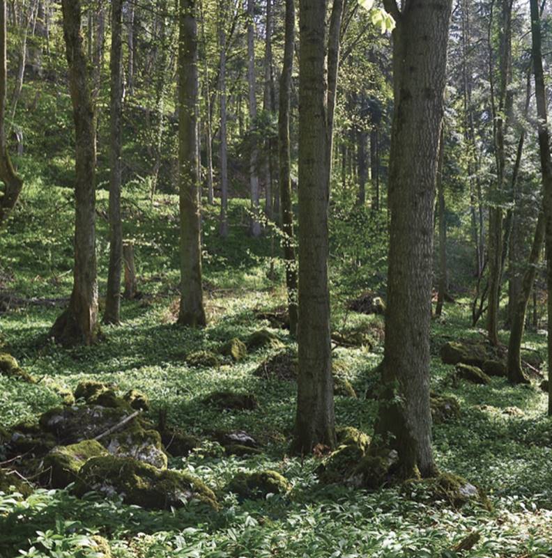
Mixed temperate forest at the Lageren, Switzerland. This forest ecosystem is located at 682 m above sea-level on a south-facing slope and is characterised by a relatively high species diversity and a complex canopy structure. It is dominated by European beech (Fagus sylvatica), but also includes species like Norway spruce (Picea abies), European ash (Fraxinus excelsior), silver fir (Abies alba) and sycamore maple (Acerpseudoplatanus). This diverse forest grows on rendzic leptosols (or rendzinas) and haplic cambisols which have developed on limestone and marl and already start less than one metre below the soil surface. In spring, a lush understory of wild garlic (Allium ursinum) is present

A terrestrial ecosystem includes the soil, microorganisms (both in the soil and aboveground), vegetation and animals as well as the lower level of the atmosphere, all interacting with each other. Terrestrial ecosystems are functional units in a given heterogeneous landscape and are present in all climatic zones, ranging from tropical forests to arctic tundra. Their size ranges from a couple of square metres, for example a dwarf heather ecosystem at alpine elevations, to a couple of square kilometres, for example a uniform agricultural field or a boreal coniferous forest. In any case, terrestrial ecosystems are the functional unit where biogeochemical processes happen, such as nitrogen mineralisation, where these processes provide the necessary inputs, such as plant available nitrogen forms, to ensure plant performance, such as growth, and where organisms compete with each other and interact with their environment.

In addition, terrestrial ecosystems must also be considered thermodynamically “open” ecosystems, where water and nutrients get lost, for example as emissions to the atmosphere or via leaching and run-off, thereby also affecting the environment. Terrestrial ecosystems are also the management unit that agriculture and forestry use (Part V: Global Ecology). Thus, terrestrial ecosystems are the organisational unit where processes such as primary productivity and water use need to be understood to predict the impacts of natural and anthropogenic disturbances on the provisioning of services, such as food and timber production.

The science of (terrestrial) ecosystem ecology has grown considerably over the last several decades. Various scientific approaches are being used, ranging from classical observations to manipulation experiments, from plot to continental scales, from empirical or statistical modelling to dynamic vegetation models combined with biogeochemistry models. Over the last several decades, measurement techniques used in ecosystem ecology have been developed and improved tremendously, adding techniques from formerly neighbouring disciplines as well, nowadays for example including high-tech systems to measure biospheric-atmospheric greenhouse gas fluxes and their isotopic signatures as well as remote sensing techniques used on airborne platforms or at tall towers.

Terrestrial ecosystem ecology draws on many disciplines, from soil science and hydrology, microbiology, animal and plant sciences to meteorology and atmospheric sciences. However, the link between community ecology (Part IV; mainly focusing on environmental effects on communities and community dynamics) and ecosystem ecology (mainly focusing on pools and fluxes) has only developed over the last decade, triggered by the wish to understand how species and communities, affected by environmental change, in turn affect ecosystem processes and services. Thus, ecosystem ecology is truly interdisciplinary, that is scientists from different disciplines work together to jointly address their research objectives. Sometimes ecosystem scientists even reach out to stakeholders, such as farmers, foresters, nature conservationists or politicians, and therefore ecosystem ecology has become transdisciplinary.

Here we will focus on terrestrial ecosystems, neglecting aquatic ecosystems on land, such as rivers or lakes (i.e. freshwater systems). We will consider managed and unmanaged ecosystems, the latter sometimes erroneously called “natural” ecosystems, although most ecosystems on Earth are managed in one way or another, from agricultural production to protection for nature conservation. Furthermore, all ecosystems are affected by environmental and human drivers, independent of management. Thus, we must realise that all global ecosystems are affected by human activities, even very remote ones (Part V).

We will first explain the concept of an ecosystem and describe the characteristics of a terrestrial ecosystem as functional, not as hierarchical unit (Chap. 13: Ecosystem Characteristics). Then different approaches will be illustrated that are used to study terrestrial ecosystems, and insights into representative ecosystem studies will be given (Chap. 14: Approaches to Study Terrestrial Ecosystems). We will then give an overview about ecosystem modelling (Chap. 15: Approaches to Model Processes at the Ecosystem Level). Finally, a process-oriented view will be adopted, and selected biogeochemical fluxes into, within and out of terrestrial ecosystems will be discussed, such as those of water, carbon and nitrogen, as well as nutrients (Chap. 16: Biogeochemical Fluxes in Terrestrial Ecosystems).