Carbon Fluxes in Terrestrial Ecosystems

Carbon Pools and Fluxes in Terrestrial Ecosystems. Carbon enters terrestrial ecosystems as atmospheric carbon dioxide (CO₂) during gross primary production (Fig. 16.11). It is allocated as carbohydrates within plants and used to grow plant tissues and for storage, but also to fuel ecosystem respiration, both from autotrophic plants and heterotrophic microbial organisms and soil fauna. Because of these two large ecosystem CO₂ fluxes (photosynthesis and respiration), there is a close coupling between the atmosphere and the biosphere, mediated by a turbulent exchange of air masses above and within the ecosystem.

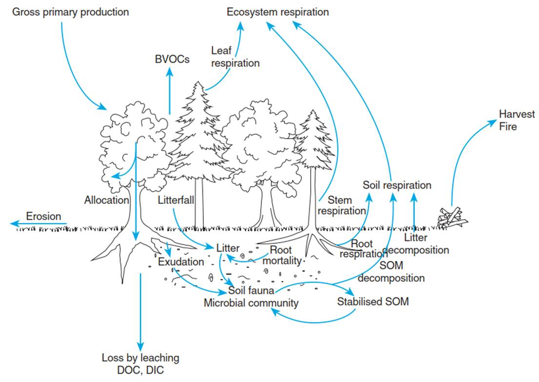
Fig. 16.11. Carbon pools and fluxes in terrestrial ecosystems. Carbon enters the ecosystem as carbon dioxide via photosynthesis and leaves the system as carbon dioxide via autotrophic (root, stem, foliage) and heterotrophic (microbial, soil fauna) respiration. Further carbon losses occur as leaching of dissolved organic and inorganic carbon (DOC and DIC, respectively) as well as via erosion. Additional losses result from harvests and fires

When plant tissues senesce and become litter, decomposition of this dead organic matter (necromass) sets in. Decomposition by soil fauna and microorganisms includes decay, that is, the biotic breakdown of organic matter, and mineralisation, that is, the release of inorganic nutrients, but also CH₄ and CO₂ (thus het- erotrophic respiration). Stabilisation of organic matter, that is, the formation and protection of soil organic matter (SOM), contributes to carbon sequestration. Thus, the largest carbon pool in ecosystems is often in the soil (except in tropical forests).

Additional losses occur during leaching of DOC and dissolved inorganic carbon (DIC) from the soil, but also during erosion. During fires and with harvests, large amounts of carbon are removed from ecosystems, although both fire and harvest residues also make large contributions to SOM. Depending on fire frequencies and the degree of ecosystem management, vegetation degeneration, soil degradation and erosion can occur. For the exchange of methane (CH₄) and other biogenic volatile organic compounds (BVOCs).

One variable often used to address ecosystem carbon budgets is net primary production (NPP), in g C m^-2 year^-1, defined as GPP minus respiration. Thus, it includes, for example, production of fine roots, root exudation and emission of BVOVs for defence. NPP constitutes about 50% of GPP (ranging from 30% to 80%) (Amthor 2000; DeLucia et al. 2007) and can be determined for above-ground and belowground tissues (ANPP and BNPP, respectively). Moreover, allometric relationships (i.e. statistical relationships used to predict tree biomass) relate BNPP to total NPP. For example, for trees BNPP/NPP = 0.3, and for grasses BNPP/ NPP = 0.5. These numbers are global means and thus do not account for species differences. Moreover, most NPP estimates given in the literature are ANPP estimates only, neglecting below-ground production but also herbivory and other processes like exudation and BVOC emissions.

Thus, NPP should not be interpreted as yield, harvest or above-ground biomass production over time (e.g. ANPP per growing season, cropping time, year). Two examples illustrate this misconception: Farmers consider grain production as yield but are not necessarily interested in stem and root growth; foresters are mostly interested in cumulative stem growth and increase in wood volume at time of harvest but not in foliage growth or even stem mortality until harvest. Moreover, thinning and harvest residues are clearly part of NPP but not considered in assessments of net increment changes in forests. Both examples illustrate that the harvestable yield is only a small fraction of NPP.

Moreover, there exists no direct relationship between standing biomass (in g C m^-2) and NPP (in g C m^-2 year^-1). Biomass produced by plants persists at the plant or in the ecosystem for very different time periods, leading to different values of standing biomass due to function (e.g. wood) and tissue longevity (Table 16.2). For annual species, the total biomass dies off at the end of the growing season (except seeds) and serves as substrate for heterotrophic organisms in the soil. For perennial herbaceous plants, almost all the total biomass produced also dies (except rhizomes, bulbs or corms, i.e. underground stem storage organs) and becomes litter within a year. Thus, for herbaceous species, this litter production corresponds to ANPP.

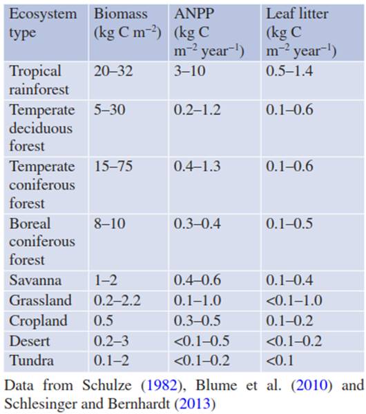
Table 16.2. Standing biomass, above-ground net primary production (ANPP), and leaf litter production in different ecosystem types

In contrast, in woody plants, about 50% of ANPP is invested in wood. Part of the sapwood is subsequently transformed into dead heartwood, which becomes woody debris and litter only with a long time delay. Moreover, only about 40 to 50% of deciduous tree ANPP and about 20% of evergreen tree ANPP reaches the soil each year as leaf, twig and root litter. Thus, neither standing wood biomass nor litter fall reflects annual NPP or ANPP in forests.

A large proportion of total biomass is belowground and thus “out of sight”. Therefore, information about standing biomass, production and mortality, thus turnover, is more difficult to obtain than for above-ground biomass. On average, the proportion of fine roots as part of total biomass is about 28% (Table 16.3). Fine roots in forests reach a total length of 2-8 km m^-2 and a projected area of 4-11 m² m^-2, corresponding in magnitude to the LAI. In grasslands, the length of fine roots (>100 km m^-2) is a factor of 10 greater than in forests. The NPP of fine roots probably corresponds to the turnover of leaves.

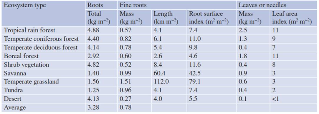
Table 16.3. Biomass of fine roots (<2 mm diameter) and leaves in different ecosystem types on Earth (Data from Schulze 1982; Jackson et al. 1997)

Thus, estimating NPP is difficult for different reasons. Plants might be difficult to reach or to measure, for example, tropical trees, epiphytes and lianas; some processes, particularly in the soil, might be difficult to determine, for example, root exudation or production and turnover of fine roots (<2 mm diameter). For example, different methods exist to estimate fine root biomass production and turnover, ranging from

- Sequential root biomass sampling.
- Ingrowth cores: mesh bags filled with root- free soil, placed into the rooting zone, and collected after some time to quantify the new roots grown into the cores.
- Minirhizotrons: cameras inserted into the soil to monitor root growth with transparent tubes.
- Stable isotope labelling: tracing the fate of ¹³C-labelled photoassimilates into root growth.
- Radiocarbon dating based on bomb-carbon: ¹⁴C created by above-ground nuclear tests done in the 1950s and 1960s (also called bomb-carbon), recovery of bomb-carbon in tissues, compounds or ecosystem compartments, relationship to decreasing atmospheric ¹⁴C background values and thus to the age of the C analysed.

Each method has its own uncertainties, but generally sequential coring and minirhizotron estimates seem to overestimate turnover, while radiocarbon analyses seem to underestimate turnover (Gaul et al. 2009). Consequently, estimates of mean life span for the same fine roots might differ. In temperate forests, life spans of typically <1-2 years were found based on sequential coring and minirhizotron methods. However, fine root life spans were much larger, up to 8 years (top soil) and 18 years (deeper soil horizons), based on radiocarbon analyses (Gaudinski et al. 2001).

However, radiocarbon estimates can be biased, depending on which carbohydrate substrates with which age (i.e. time since bomb tests) are used for fine root production. Clear evidence was provided by Vargas et al. (2009) using radiocarbon analyses in five tropical forest stands before and after Hurricane Wilma hit. Fine roots grown into ingrowth cores installed after the hurricane were estimated to be 2-10 years old. Thus, trees had remobilised stored, that is, old, carbohydrates to supply new fine root production and did not use recently assimilated carbon.

This made new roots look much older! Independently of the method used, most studies find thicker and deeper roots being older than fine roots in the top soil. Root turnover differs among different ecosystem types. For example, fine root turnover in grasslands is typically much greater than in forests, that is, the life span of fine roots in grasslands is much shorter. In comparison, leaves and needles in temperate forest ecosystems have a life span of 1-10 years (Pinus aristata even 30 years). Wood can remain at a plant >100 years (oldest living trees: 5000 years, Pinus longaeva, Bristlecone pine), while SOM is often >100- 1000 years old.

One of the largest CO₂ fluxes in terrestrial ecosystems is soil respiration (also called soil CO₂ efflux), comprising between 50 and 70% of total ecosystem respiration (Raich and Schlesinger 1992). Soil respiration includes respiratory losses from plants and plant-root-related microorganisms in the rhizosphere, microbial respiration (MR) during decomposition of litter and SOM as well as respiration of soil fauna (Fig. 16.12).

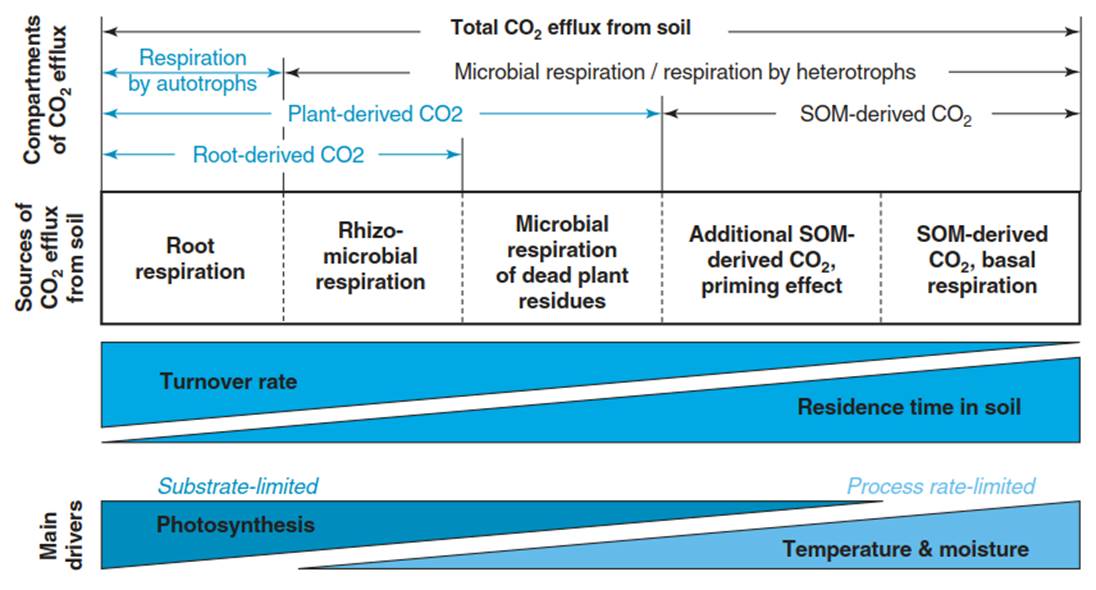
Fig. 16.12. Processes and organisms contributing to soil respiration in the form of soil CO₂ efflux to total ecosystem respiration. Turnover rates and, thus, residence times of the substrates differ among the different component fluxes, as do the main drivers. (Kuzyakov and Gavrichkova 2006)

The strict separation into auto- and heterotrophic soil respiration is not useful since MR is intricately coupled to plant activity, particularly to canopy photosynthesis, not only in the rhizosphere via root production and exudation but also via litter production. Depending on the substrates used for respiration, turnover rates and, thus, residence times in the soil differ. While roots respire relatively young carbohydrates allocated below-ground (<1 year to several years), MR use substrates from root exudation (<1 year) or organic matter, ranging in age from leaf litter (<1 year to several years) to very old SOM (decades to millennia). Thus, the drivers of soil respiration are both biotic (carbon supply via photosynthesis and allocation belowground) and abiotic (environmental conditions), but they also interact with each other. For example, with increasing temperature, not only respiration increases, but also photosynthesis and in turn allocation below-ground may increase up to a certain limit. With increasing N supply, productivity increases, but also the root:shoot ratio and the litter quality change, affecting MR during mineralisation of plant litter.

Overall, the most important driver of soil respiration is canopy assimilation. This can be seen when above-ground biomass is cut, for example, in managed grasslands, while abiotic conditions like soil temperature and moisture remain unchanged. Soil respiration drops within a couple of days and only resumes when above-ground biomass, and thus LAI, is regrown. Hogberg et al. (2001) used stem girdling in a northern pine forest to show for the first time the strong coupling of canopy photosynthesis to below-ground respiration. Girdling is the removal of the phloem in the bark of trees, which interrupts the supply with carbohydrates assimilated in the canopy to the root system. Depending on the starch pool in the roots, the drop in soil respiration occurred faster (low starch pool, end of season) when trees were girdled later in the year than when girdled in spring (still high starch pool, beginning of season). Similarly, drought slows down carbon allocation below-ground, affecting soil respiration negatively (Ruhr et al. 2009).

Thus, overall, soil respiration scales positively with GPP, NPP, LAI, litter production and carbohydrate supply below-ground. This affects both root-rhizosphere respiration (RR) and MR, which are tightly related to each other as well (Bond-Lamberty et al. 2004). Changes in phenology, co-occurring with changes in environmental conditions, thus affect soil respiration in mixed deciduous forests too (Ruehr and Buchmann 2010). During the growing season with full canopy cover, RR is greater than microbial soil respiration, contributing on average 50-60% to total soil respiration. However, during the dormant season, this contribution of RR drops to about 30%, with microbial soil respiration dominating the overall soil CO₂ flux.

Nevertheless, environmental conditions, particularly soil temperature and soil moisture, also regulate soil respiration. Since both abiotic factors also drive canopy photosynthesis and are more readily available than GPP, soil respiration is often modelled with climatic data, particularly at large spatial scales. Soil respiration increases exponentially with soil temperature, while low soil moisture contents decrease soil respiration below this general relationship. Phenology also affects these functional relationships (Fig. 16.13).

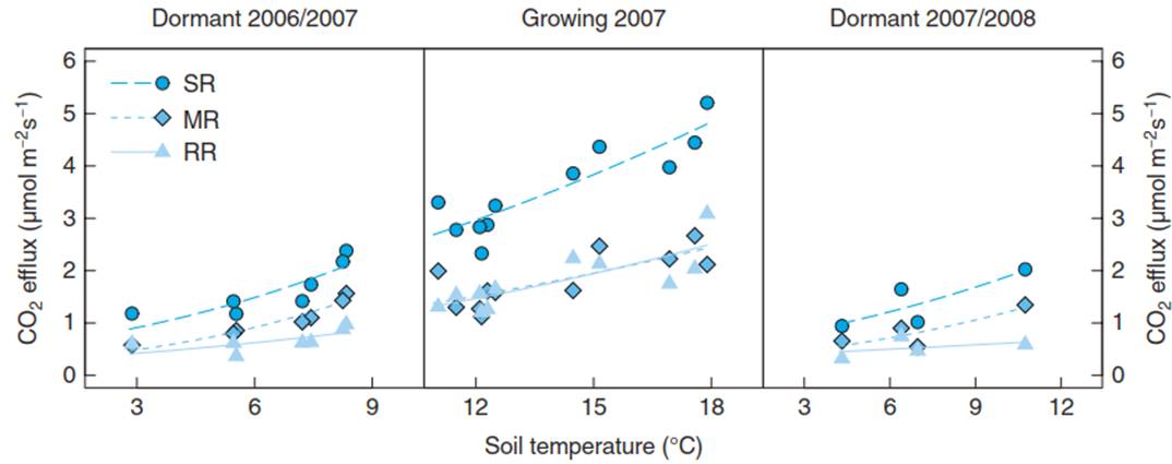
Fig. 16.13. Functional relationships of soil temperature with soil respiration (SR), microbial (MR) and root-rhizosphere respiration (RR). Fluxes were measured in a mixed deciduous forest during the dormant seasons (no tree foliage; 2006/2007 and 2007/2008) and the growing season (full canopy; 2007). SR was measured on grown forest soil. Using mesh bags, roots were excluded from the bags, and MR could be measured separately. RR was calculated by difference (RR = SR — MR). (Ruehr and Buchmann 2010)

During the growing season, both RR and MR show similar relationships with soil temperature. However, during the dormant seasons, when fluxes are lower, MR reacts more strongly to increasing soil temperatures (steeper slope) than root respiration. Most likely, RR during the dormant seasons is limited by carbon substrates compared to MR, which can use many organic matter substrates available in the soil. Owing to these interacting multiple drivers, a simple Q₁₀ value, which describes the increase of an enzymatic process when temperature is increased by 10 K, cannot capture this complexity. Thus, it should not be used to describe soil respiration fluxes in response to changing environmental drivers, not even to temperature changes alone (for further details, Davidson et al. 2006). Instead, modelling needs to take into account both environmental and biotic variables.

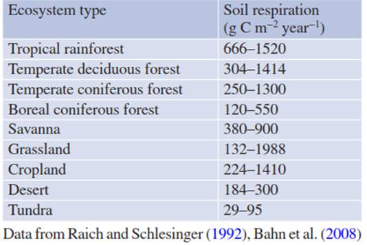
Table 16.4. Soil respiration fluxes across different ecosystem types

Based on these interacting biotic and abiotic drivers, it is not surprising that total annual soil respiration fluxes vary strongly within and across ecosystem types (Table 16.4). Soil CO₂ fluxes can be as large in grasslands and croplands as in forests. Lower plant productivity due to climate limitations results in lower soil respiration rates, such as in desert, boreal forest and tundra ecosystems.