Models of Intra- and Interspecific Competition
Any simple concept can be couched in mathematical terms, which offers completely new approaches to investigating the effects of competition for populations and communities. However, such models can “only” explore the consequences of their assumptions and, hence, must be shown to apply to any given situation. Still, the conceptual clarity such models can provide far outweighs their limitations.
The key idea in competition models is to express the competitive effects of species A on B in multiples of the effect of A on A, that is, the balance of inter- versus intraspecific competition. All else being equal, if B is twice the biomass of A, each individual of B should have twice as much effect on A as an individual of A. To be able to put this into a simple formula, we first recall that the density-dependent growth of a population of species A can be represented by a logistic equation:
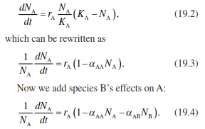
Thus, the coefficient aAA represents intraspecific competition (read: A affected by A), while aAB (read: A as affected by B, or B on A) represents interspecific competition of B on A. By analogy, we have another equation describing the population dynamics of B, which is identical apart from the indices. This set of equations is known as Lotka-Volterra competition (Case 2000). Typically, competition is not symmetric, that is, aAB ≠ aBA. The competition coefficients represent the overlap of niches between the two species: more overlap means more competition.
The coexistence of the two species is possible if either species can invade a monoculture of the other species. For example, species B can invade a monoculture of species A if the effect of A on itself is larger than that on B: aAA > aBA and aBB > aAB (Chesson 2000). In simple words: coexistence requires intraspecific competition to be stronger than interspecific competition. (Coexistence is achieved if the relative competition coef
uninformative about coexistence. We need to know how strongly the resident is affecting the invader, not how strongly it is affected by the invader!)
The Lotka-Volterra system was initially without reference to a mechanism, but it can be derived from diffuse competition for a single resource (MacArthur 1969; Tilman 1982).
It is worth recalling that intraspecific competition is density-dependent, leading to selfthinning, for example, in forest stands (Yoda et al. 1963). It is therefore not unreasonable to consider that also competition is density-dependent on competitor B and, hence, that competition coefficient aAB varies (non-linearly) with the number of individuals of B: aAB = f(NB). This makes no difference for the preceding situation, as long as we investigate only the moment of invasion (i.e. resident at equilibrium, invader at zero). For two- species systems, we can still manipulate densities across both species and determine the competition coefficients (in what is called a response surface design; Box 19.1). For multiple species, this becomes practically impossible.
One mechanistic interpretation was offered by Tilman (1982), the so-called R* rule. It states that the winning species in a competition is the one that tolerates lower resource concentrations for persistence (survival and reproduction). This lowest level is symbolised by R*, and the species with the lowest R* value wins (Box 19.2, Chap. 17)
Box 19.2: Graphical Model of Plant Coexistence Under Multiple Resources
Tilman (1982) proposed a graphical model to understand the competition of two species for two resources. A crucial feature of this model is that resources get depleted, so competition is decided in favour of the species that can survive on the lowest amount of resources. This level of minimum resource requirement is called R*, and it differs between species and resources.
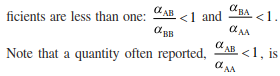
Figure 19.11 illustrates competition between species A (red) and B (blue) for resources 1 and 2. The lines (“zero-growth isoclines”) indicate the minimum requirements for the two resources. In Fig. 19.11a, species B has lower resource requirements than A for both resources (indicated by the dashed lines). In this situation, B will always deplete resources to a value below A’s requirements, so A will go extinct.
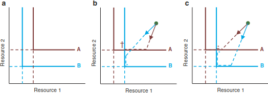
Fig. 19.11. Competition between two species for two resources. a B has lower resource requirements than A for both resources and hence wins. b Resource consumption (arrows) reduces resource 2 more than resource 1, again leading to dominance of B. c Resource requirements and consumption match, coexistence is possible. (Tilman 1982)
The situation changes if A and B have a resource for which their R* is lower than that of the other species (in Fig. 19.11b, c, R*1A < R*ib and R*2B < R*2A). This alone, however, does not guarantee coexistence. Imagine a level of resources indicated by the green point. The two species will now consume the two resources, indicated by the arrows (consumption vectors). In Fig. 19.11b, species A hits its minimum requirement of resource 2, but species B continues to exploit resource 2 below A’s R*2—and species A goes extinct.
In Fig. 19.11c, the consumption vectors are swapped: now species A consumes resource 2 slower than species B. As resource 2 is depleted to A’s minimum level, B can further deplete it. At some point (in the blue corner), resource 1 will become limiting for B. Here, its consumption of resource 2 will stop, too. As resource 2 recovers, species B cannot profit from it because it is still limited by resource 1. Hence, resource levels will move to the point where the zero-growth isoclines for the two species intersect and where both species can coexist (indicated by *).
Along a gradient of resource ratios, species with different R* values replace each other. To see that, we must extend the previous figure to more species (Fig. 19.12).
Fig. 19.12. Competition between four species for two resources. (Tilman 1982)
As the ratio of resources changes (Fig. 19.12 right: R1:R2), different pairs of species coexist at different positions of the resource-ratio gradient. In systems with spatially variable resource ratios, the coexistence of several species becomes possible.
Experimental confirmation of this concept comes from work on competition between five grass species, each lowering the concentration of soil N below the minimum requirement of their inferior competitors (Tilman and Wedin 1993). However, because such experiments are extremely laborious, the role of this theory in realised vegetation remains unclear.
Chesson (2000) made the important theoretical distinction between two different kinds of mechanisms contributing to coexistence: stabilising processes (e.g. the Janzen-Connell effect discussed subsequently) are typically linked to density dependence and allow a species to increase at low densities, thereby preventing its local extinction. Equalising processes (such as disturbance or environmental harshness) contribute to averaging out fitness differences between species; they slow down the extinction of one species by another but cannot ultimately prevent it.
The density-dependent competition effect would be a stabilising force (as low densities lead to no competition and, hence, prevent extinction), while species with similar or even identical R* values would only be equalised, but not stabilised. If, through a stochastic disturbance, one of them decreased, there is no process that would allow it to rebound to higher abundance, a mechanism required for stabilisation. Apart from the aforementioned balance of intra-interspecific competition, there are two more involved fluctuation-dependent processes, which require a variable resource: the relative non-linearity of competition and the storage effect. Note that, in general, the Lotka-Volterra system also works in variable environments, but these two new processes require such variability.
The relative non-linearity of competition describes two species whose growth rates respond differently (e.g. one linearly, the other non-linearly) to the limiting resource. As this resource fluctuates, sometimes one will grow better and be competitively superior, sometimes the other. While it is unclear how relevant this effect is in real communities, the theoretical potential for allowing coexistence among many species under multiple fluctuation resources is great (Huisman and Weissing 1999).
The second, and possibly more commonly known, fluctuation-dependent stabilising mechanism is the storage effect. It actually requires that three assumptions be met: (1) species must respond differentially to the environment; (2) competition must be driven by the environment, such that growth and competition co-vary; and (3) poor growth conditions must be tolerated, for example, population growth must be buffered (e.g. by seed banks). The “spatial” storage effect occurs when competing plant species grow in monospecific patches, so that each species has conditions in which it thrives and those in which it is subdued. The “temporal” storage effect is exemplified by spring geophytes in deciduous forests (such as wild garlic Allium ursinum, lesser celandine Ranunculus ficaria, wood anemone Anemone nemorosa) (Sect. 9.2, Chap. 9). Spring geophytes emerge in late winter or early spring and use the period before trees regrow their foliage. They then translocate their nutrients into below-ground storage organs, awaiting the next season.
Apart from these coexistence mechanisms, there is also an important spatially explicit coexistence mechanism: the competition-colonisation trade-off. The premise of the competition-colonisation trade-off is that plant species are either good colonisers or good competitors in the establishment phase (Slatkin 1974). An obvious trait to look at would be seed size: small seeds are dispersed more readily and over larger distances, while large-seeded species will have an easier time germinating and living off the seed’s resources for longer. In this way small- seeded species will find empty patches in a wider part of the landscape, while large-seeded species will only disperse close to the mother plant but dominate over the smaller-seeded species there. Coexistence is achieved at the landscape scale, and over multiple generations, rather than in any given patch at any time (if at all: the competition-colonisation trade-off is an equalising mechanism, not a stabilising one). While this mechanism resembles the r-K strategies, it is a bit more specific and, hence, more readily testable. Experimentally, the benefit of large seeds is difficult to verify, and recently the ability of large seeds to tolerate droughts and shade has been proposed as a more plausible mechanism (Muller-Landau 2010).
In recent years, neutral mechanisms of coexistence have become more prominent (Hubbell 2001) (Fig. 19.13). Neutral refers to the assumption that species (e.g. within a functional group or guild) are equivalent in all aspects relevant for competition, such as dispersal, competitive strength and so forth. In such a situation, a species filling a vacant patch in the community is drawn randomly from the species pool, as in a lottery. Over many generations, this will lead to “ecological drift” in community composition, sometimes one, sometimes another species being most abundant, and rare species going extinct. Unless new species are added from outside, eventually only one species will remain, but which one cannot be predicted. Such lottery competition is an old theoretical hypothesis of coexistence, which does not chime well with our current understanding of stabilising and equalising mechanisms and remains difficult to test because of its long-term prediction and high stochasticity.
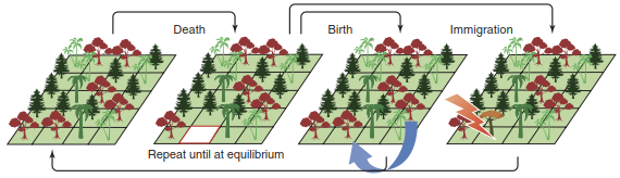
Fig. 19.13. Neutral community dynamics. All species are assumed to be equivalent to each other; death, birth and immigration processes are purely stochastic. Such neutral dynamics lack stabilising processes and hence do not lead to coexistence. Thus, any given local community will display species turnover (“ecological drift”), with amount and distance of dispersal and the size of the entire community determining local species richness (Rosindell et al. 2011). Reproduced with permission from Elsevier
Finally, we shall be looking at competition and coexistence involving other trophic levels, such as the Janzen-Connell effect, in Sect. 19.3.3.1.
Date added: 2026-04-26; views: 162;