Algorithms to Reduce the Computational Cost Associated to the RSQ

The computational costs of RSQ have directed research to develop many powerful algorithms, some of which will be summarized here. It is important to note that the aim of these algorithms is to only reduce the cost associated to the second sub-problem described in the section on the Problems and complexity of RTT.

These algorithms only address the shadowing problem (which appears in both SBR and SIP) and their application is the same, independent of the ray mechanism. The searching of the ray path associated to these mechanisms is not improved by these algorithmic techniques.

RSQ algorithms are usually applied in a preprocessing phase and in an execution phase. In the preprocessing phase, the input data structure that contains the information of the entities (usually facets) that define the geometry is reorganized. This reorganization groups close and/or visible geometrical entities together in the data structure, and/or relations of proximity or visibility are associated to the appropriate entities.

The simplest RSQ algorithm encloses completely each entity of the scene in a bounding box, preferably in a parallelepiped of minimum volume, with sides perpendicular to the Cartesian absolute system chosen to represent the geometry (see Fig. 7).

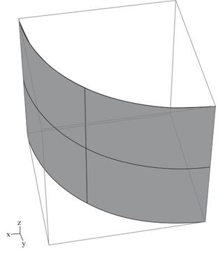
Figure 7. Example of the bounding box that encloses a curved surface

The bounding box RSQ is compatible with other RSQ algorithms. It is performed as follows: Before checking the intersection of the ray with the curved facet, by means of a rigorous checking procedure, it is determined if a ray impacts the box. Obviously, the ray cannot be occluded by the surface if the check is negative. This surface is not considered in the shadowing test, which avoids more time-consuming procedures for checking the possible intersection of the ray with the facet.

Most RSQ algorithms are based on a volumetric spatial partition (VSP) of the scene. After this division, the scene is split into small subvolumes that contain groups of scene entities, with some subvolumes potentially empty. To determine whether a segment is occluded by one or more scene entities, we only need to check the entities contained in the subvolumes that the segment crosses.

Figure 8 shows an example of the division of a simple two-dimensional (2-D) scene in voxels. An example of the ray tracing between a source (S) and an observation point (O) is depicted in the figure. It can be noted that only the entities contained in the voxels that the ray crosses are involved in the RSQ, which reduces the complexity of this task.

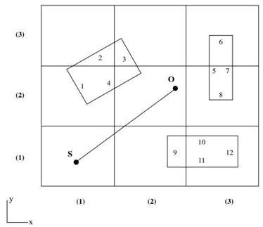
Figure 8. Example of the application of the SVP for a simple 2-D scene. The scene is divided in voxels

Many efficient RSQ algorithms are based on VSP. The major difference between these algorithms is the strategy used for space division, which can significantly impact final algorithm efficiency. One of those algorithms is binary space partitioning (BSP). BSP requires the space to be divided into subvolumes in successive steps such that each subvolume is split in two halves (binary partitioning). The BSP has two versions. In the polygon-aligned version, the space subdivision in two halves is made considering the regions above and below each flat facet of the scene.

This version is not applicable when the scene has curved surfaces. In the axis-aligned version, a division into two halves of a subvolume is made by a plane perpendicular to the Cartesian coordinate system that defines the scene.

Figure 9 shows the application of the axis-aligned version of BSP to a simple 2-D scene, and Fig. 10 presents the associated BSP tree. The subdivision in a level tree is perpendicular to a coordinate axis; the axes alternate in consecutive tree levels. Each node of the BSP tree corresponds to a division of a subvolume.

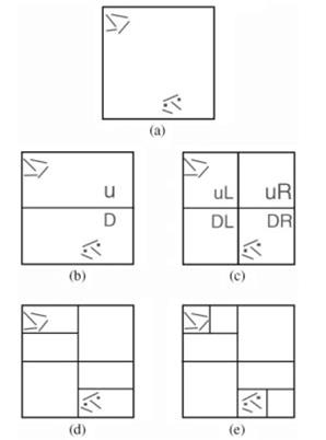
Figure 9. Example of spatial partition of and scene using the BSP axis-aligned technique. The scene has only two groups of entities, which are indicated by the small straight lines in the top and in the bottom of the scene rectangle

When a subvolume is empty, it is not subdivided, and its tree node becomes a tree leaf. This tree is very helpful in the RSQ because, to determine the intersection of a ray segment with one of the entities of the scene, only the entities that belong to the low-level subvolumes of the BSP tree that the segment crosses. For example, in Fig. 10, if a segment joins two solid points in the subvolume ofnode DRDL when applying the BSP, only the entities in the subvolume DRLD must be checked, obviously reducing considerably the number of intersection tests to be performed.

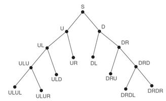
Figure 10. BSP tree for the case of Fig. 6

Today, one of the most efficient algorithms for solving the RSQ is the kd-tree algorithm, which is similar to the axis-aligned version of the BSP. The difference between these algorithms is that, during the preprocessing phase of the kd-tree, the subvolumes in each binary division do not necessarily have the same size. The size of the subvolumes is fitted to give the bigger size to the empty or less populated subvolume.

Octree Space subdivision is another technique for solving the RSQ that is similar to the BSP, except that now each subvolume is split into eight small subvolumes (called octrees) by the three coordinate planes. Other variants of the VSP are the division of the scene volume into a uniform grid of equal-sized sub-volumes. Simultaneously, each subvolume can be split into a new grid of uniform sub-volumes. This process can be repeated several times to form hierarchical grids.