The Role of Terrestrial Ecosystems and the Ocean in the Global Carbon Cycle

Coupling of Climate and Biosphere Through the Carbon Cycle. Terrestrial ecosystems are tightly linked to the climate system not only through biogeophysical feedbacks (energy and water cycles), but also via the global carbon cycle. The terrestrial biosphere absorbs a significant portion of annual anthropogenic carbon dioxide (CO₂) emissions. This carbon-sequestration effect is driven by the stimulation of photosynthesis under rising atmospheric CO₂ concentrations and changing climate, increased nitrogen deposition, and forest recovery on abandoned agricultural lands.

Over long timescales, geographic shifts in biomes and changes in ecosystem biogeography substantially alter land carbon storage capacity. According to climate modeling results, the land carbon cycle forms a positive feedback loop: global warming reduces the terrestrial biosphere's capacity to absorb and retain anthropogenic emissions. Uncertainty in carbon cycle feedback projections is comparable in magnitude to the uncertainty in physical climate processes. This stems from physiological responses of plants and microorganisms to temperature changes, as well as vegetation demographic responses to disturbances and climatic shifts. Furthermore, because productivity in many terrestrial ecosystems is nitrogen-limited, strong carbon-nitrogen interactions occur, including:

· Constrained productivity growth under atmospheric CO₂ enrichment;

· Enhanced productivity driven by nitrogen deposition;

· Additional nitrogen mineralization resulting from soil warming.

CO₂ Dynamics in Glacial–Interglacial Cycles. Under natural conditions, absent anthropogenic influence, atmospheric CO₂ levels are governed by the balance between oceanic and terrestrial processes. Over hundreds of thousands of years, atmospheric CO₂ concentrations fluctuated within a ~100 ppm range across glacial and interglacial cycles (see Figure 8.2). During glacial periods, CO₂ levels were markedly lower (~180–200 ppm) than during interglacials (~270–290 ppm). While the underlying causes of these fluctuations are not fully resolved, oceanic processes play a key role (Ciais et al. 2013). Specifically, the colder glacial ocean stored more carbon due to the increased solubility of CO₂ at lower water temperatures. Changes in ocean circulation further contributed to lowering atmospheric CO₂, whereas sea level drop and increased salinity in the glacial ocean acted in opposition to reduce oceanic carbon storage.

In contrast to the ocean, carbon storage in the terrestrial biosphere decreased during glacial periods. Studies of the Last Glacial Maximum (18,000–21,000 years ago) reveal a biosphere fundamentally different from today's. Desert and semi-arid shrubland biomes expanded substantially, while boreal and temperate forest areas contracted. Dry woodlands and savannas displaced humid tropical forests. The biomes dominating under cold and arid glacial conditions were characterized by low carbon storage per unit area, indicating a smaller total terrestrial carbon pool compared to the present interglacial. Estimates of this terrestrial carbon deficit range from 300 to 1,000 Pg C (Prentice et al. 2011; Ciais et al. 2013).

Holocene Stability and the Anthropogenic Shift. Throughout the current interglacial (the Holocene), prior to the industrial era, atmospheric CO₂ concentrations remained relatively stable. Over the past 11,000 years, CO₂ hovered between 260 and 280 ppm, increasing by approximately 20 ppm over the 7,000 years preceding the industrial era, as illustrated in Fig. 29.1. The driver of this modest variation is attributed to ocean chemistry changes (leading to CO₂ outgassing) and, to a lesser extent, shifts in the terrestrial biosphere (Ciais et al. 2013). High-precision ice core data show minimal CO₂ fluctuations during the last millennium up to 1750 (see Fig. 29.2), with the exception of a brief decline of ~10 ppm around 1600.

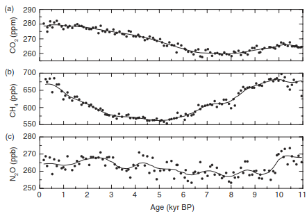
Fig. 29.1. CO₂ (a), CH₄ (b), and N₂O (c) concentration over the Holocene from the EPICA Dome C ice core in Antarctica. Data from Flückinger et al. (2002) and Monnin et al. (2004) and provided by the National Climatic Data Center Paleoclimatology program (National Oceanic and Atmospheric Administration, Boulder, Colorado).

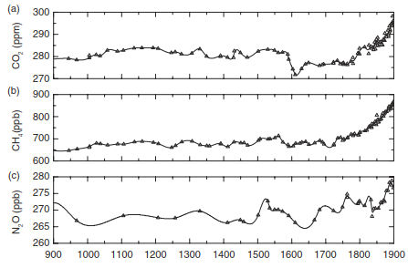
Fig. 29.2. CO₂ (a), CH₄ (b), and N₂O (c) concentration over the period 900–1900 from the Law Dome ice core in Antarctica. Data from MacFarling Meure et al. (2006) and provided by the National Climatic Data Center Paleoclimatology program (National Oceanic and Atmospheric Administration, Boulder, Colorado).

Modern Carbon Budget and Balance. Atmospheric CO₂ levels in the modern era reflect the balance between anthropogenic emissions from fossil fuel combustion, industrial processes, deforestation, and land-use change versus the carbon sinks in the ocean and land biosphere. During the industrial era, atmospheric CO₂ rose by over 40%: from 278 ppm in 1750 to 390 ppm in 2011 (Table 2.1, Figure 3.7a). Human activities emitted 555 ± 85 Pg C through fossil fuel combustion, cement production, and land-use change (Table 29.1). However, less than half of this total—43% (240 ± 10 Pg C)—accumulated in the atmosphere. The ocean and terrestrial biosphere absorbed the remainder in roughly equal measure. Analysis of data spanning 1960–2010 confirms that approximately 45% of total emissions remained airborne (Ballantyne et al. 2012; Le Quéré et al. 2013).

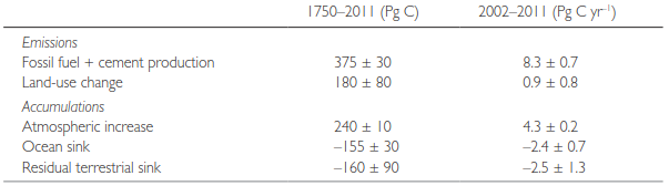
Table 29.1. Global carbon budget over the industrial era (1750–2011) and for the 10-year period 2002–2011. Note: Data for the industrial era are cumulative fluxes. Data for 2002–2011 are annual fluxes averaged over the ten years. Positive values denote carbon sources. Negative values denote carbon sinks. Source: From Ciais et al. (2013).

The 2002–2011 decade clearly illustrates the structure of the modern global carbon cycle (Table 29.1):

· Annual carbon input from fossil fuels and cement production reached 8.3 ± 0.7 Pg C yr⁻¹.

· Land-use change contributed an additional 0.9 ± 0.8 Pg C yr⁻¹.

· The atmospheric carbon accumulation rate was 4.3 ± 0.2 Pg C yr⁻¹ (about half of total anthropogenic emissions).

· The remaining 4.9 Pg C yr⁻¹ was sequestered by the ocean and land biosphere.

· The net ocean flux was -2.4 ± 0.7 Pg C yr⁻¹ (negative values indicate oceanic uptake).

· The residual terrestrial sink was -2.5 ± 1.3 Pg C yr⁻¹ (unconverted land ecosystems accumulated carbon).

· The net land–atmosphere flux (-1.6 ± 1.0 Pg C yr⁻¹) represents the difference between land-use emissions and the residual land sink driven by global environmental changes (rising CO₂, warming, nitrogen deposition).

Decadal Trends and Sink Uncertainties. Figure 29.3 illustrates the decadal variability of the global carbon cycle over the past 50 years. Emissions from fossil fuels and cement expanded 2.5-fold: from 3.1 ± 0.2 Pg C yr⁻¹ in the 1960s to 7.8 ± 0.4 Pg C yr⁻¹ in the 2000s. Land-use emissions remained relatively stable (1.5 ± 0.5 Pg C yr⁻¹ between 1960–1999) before declining to 1.0 ± 0.5 Pg C yr⁻¹ in the 2000s. The atmospheric growth rate accelerated from 1.7 ± 0.1 Pg C yr⁻¹ in the 1960s to 4.0 ± 0.1 Pg C yr⁻¹ in the 2000s. Simultaneously, ocean and land sinks increased: the ocean sink grew from 1.2 ± 0.5 to 2.4 ± 0.5 Pg C yr⁻¹, while the land sink rose from 1.7 ± 0.7 to 2.4 ± 0.8 Pg C yr⁻¹.

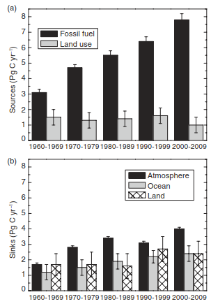
Fig. 29.3. Decadal mean global carbon budget, 1960–2009. (a) Anthropogenic emissions. (b) Atmospheric growth rate and oceanic and terrestrial sinks. Data from Le Quéré et al. (2013).

Terrestrial carbon budget estimates retain significant uncertainty because direct measurement of annual fluxes at global scales is impossible. The residual land sink is often inferred indirectly as the difference between emissions, atmospheric growth, and the ocean sink (Le Quéré et al. 2013; Ciais et al. 2013). Atmospheric CO₂ inversion models help estimate regional fluxes, but their accuracy depends on atmospheric transport modeling. Forest inventories (Pan et al. 2011) yield direct biomass measurements, though their extrapolation is constrained by spatial coverage. Eddy covariance towers measure net ecosystem productivity directly, yet their footprint remains localized (Beer et al. 2010; Jung et al. 2011). Global terrestrial biosphere models bridge local and global scales by evaluating gross primary productivity, ecosystem respiration, and land-use sinks (Le Quéré et al. 2009, 2013; Ciais et al. 2013; Piao et al. 2013).

Dynamics of Atmospheric CO₂ and Terrestrial Carbon Cycling

Atmospheric CO₂ Seasonality and Terrestrial Ecosystem Dynamics. Seasonal dynamics of terrestrial metabolism. The metabolic activity of terrestrial ecosystems is directly reflected in atmospheric CO₂ concentrations. At Mauna Loa, Hawaii, for example, CO₂ concentration has a pronounced annual cycle and varies by several parts per million (ppm) over the course of a year, with high concentration in winter and low concentration in summer, as shown in Fig. 29.4. This fluctuation occurs in response to the seasonal growth of terrestrial ecosystems worldwide, which absorb CO₂ during the growing season and respire CO₂ during the dormant season.

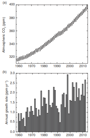
Fig. 29.4. Atmospheric CO₂ concentration measured at Mauna Loa, Hawaii, from 1959 to 2012. (a) Monthly mean concentration. (b) Annual growth rate. Data provided courtesy of Pieter Tans (National Oceanic and Atmospheric Administration, Boulder, Colorado) and Ralph Keeling (Scripps Institution of Oceanography, La Jolla, California).

Latitudinal variations in seasonal oscillations. The seasonal pulse of CO₂ occurs throughout the Northern Hemisphere, as illustrated in Fig. 29.5. The annual amplitude of the atmospheric CO₂ cycle (i.e., the difference between maximum and minimum concentrations) is greatest in high latitudes of the Northern Hemisphere and declines with latitudes closer to the equator. In the Southern Hemisphere, there is less land, oceans dominate atmospheric CO₂ exchange, and there is little seasonal variation in atmospheric CO₂.

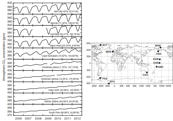
Fig. 29.5. Monthly mean atmospheric CO₂ concentration measured at 10 locations for seven years spanning 2006 to 2012. The map shows station locations. Data are from the Earth System Research Laboratory Global Monitoring Division (National Oceanic and Atmospheric Administration, Boulder, Colorado) air sampling network.

Ecosystem drivers of amplitudinal variations. Satellite and modeling analyses indicate that the annual amplitude in the Northern Hemisphere primarily reflects the seasonality of terrestrial net ecosystem production (NEP) (Tucker et al. 1986; Randerson et al. 1997; Graven et al. 2013). Boreal forests contribute greatly to the annual amplitude at high latitudes. In these ecosystems, the timing of photosynthesis and respiration is asynchronous, with photosynthesis restricted to a short growing season while respiration occurs year-round. Grasslands and croplands also have large influence, becoming increasingly important in middle and tropical latitudes. Tropical forests contribute minimally to the annual amplitude throughout much of the Northern Hemisphere, in part because of little seasonality of ecosystem processes.

Long-Term Trends and Climate Driving Mechanisms. Amplification trends in atmospheric CO₂ cycles. Temporal changes in the amplitude and seasonality of the atmospheric CO₂ cycle are important indicators of changes in the activity of terrestrial ecosystems. For example, the annual amplitude of atmospheric CO₂ concentration at Barrow, Alaska, has increased since the early 1960s, as has that at Mauna Loa, though to a lesser extent, as shown in Fig. 29.6. A large increase in amplitude is seen throughout the Northern Hemisphere north of 45° N (Graven et al. 2013). This reflects a stimulation of metabolic activity by temperate and boreal forests with greater CO₂ drawdown during the growing season (Randerson et al. 1999; Buermann et al. 2007; Barichivich et al. 2013; Graven et al. 2013). Additionally, intensification of agriculture and increased crop productivity has likely increased the amplitude of atmospheric CO₂ over the past several decades (Gray et al. 2014; Zeng et al. 2014).

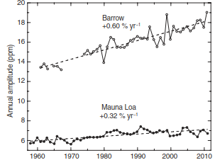
Fig. 29.6. Trends in annual cycles of atmospheric CO₂ at Barrow and Mauna Loa. Data from Graven et al. (2013).

Impact of El Niño-Southern Oscillation on terrestrial carbon fluxes. By affecting photosynthesis, respiration, and fire, climate variability exerts a discernible signal in the global carbon cycle. This is seen in the effects of the El Niño-Southern Oscillation (ENSO) on terrestrial carbon fluxes. There is an enhanced source of carbon from the biosphere to the atmosphere during warm, dry El Niño years, as shown in Fig. 29.7. This is also seen in annual atmospheric CO₂ growth rates, which are generally high during El Niño and low during La Niña.

Fig. 29.7. Global carbon flux anomalies for the period 1981–2010 for net land–atmosphere (solid line) and ocean–atmosphere (dashed line) fluxes. Light gray shading indicates El Niño events, and the dark shading denotes the anomalously cool period following the Mount Pinatubo eruption. A positive flux indicates a larger than normal source of carbon to the atmosphere, or a smaller sink. Adapted from Ciais et al. (2013).

Wildfires and satellite vegetation indices. ENSO-driven variability in the terrestrial biosphere is seen also in satellite vegetation indices (Buermann et al. 2003). Regional drought and large wildfires contribute to the high CO₂ growth rates during El Niño episodes. During the 1997 to 1998 El Niño, wildfires emitted 2.1 Pg C, or 66 percent of the atmospheric CO₂ growth rate anomaly (van der Werf et al. 2004).

Modeling primary production and satellite metrics. Production efficiency models provide a means to derive historical net primary production (NPP) using satellite and meteorological data. The normalized difference vegetation index (NDVI) gives a measure of the fraction of photosynthetically active radiation absorbed by plants. Global meteorological analyses of temperature, vapor pressure, and solar radiation provide the meteorological constraints to production efficiency. Nemani et al. (2003) and Hashimoto et al. (2004) used a production efficiency model to derive net primary production for the 1980s and 1990s and its relationship with ENSO. Their results show that global net primary production on land decreased during El Niño events with corresponding increases in atmospheric CO₂ growth rate, as shown in Fig. 29.8. This is particularly evident in 1982–1983, 1986–1987, and 1997–1998. Much of this variability originates in tropical ecosystems.

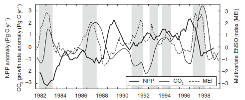
Fig. 29.8. Global net primary production (NPP) and CO₂ growth rate during the period 1982–1999 in relation to the multivariate ENSO index (MEI). NPP and CO₂ are shown as anomalies. High MEI indicates the warm phase of ENSO. Highlighted in gray are El Niños of 1982–1983, 1986–1987, 1991–1992, 1993, 1994–1995, and 1997–1998. Adapted from Hashimoto et al. (2004). See also Nemani et al. (2003).

Volcanic Aerosols and Terrestrial Carbon Sink Dynamics. Impact of volcanic eruptions on atmospheric CO₂. The period 1991–1993 is an exception to the general relationship between ENSO and atmospheric CO₂. The eruption of Mount Pinatubo in June 1991 resulted in a lower than expected atmospheric CO₂ growth rate because of enhanced net uptake by the land, and atmospheric CO₂ exhibits variability on interannual to decadal time scales due to large volcanic eruptions (Jones and Cox 2001; Brovkin et al. 2010; Sarmiento et al. 2010; Frölicher et al. 2013). Atmospheric CO₂ is generally lower than expected following large volcanic eruptions. Colder temperatures following eruptions decrease net primary production. However, the injection of volcanic aerosols into the atmosphere also increases the proportion of diffuse solar radiation.

Mechanisms governing volcanic light scattering. Diffuse radiation penetrates more deeply into a canopy than does direct beam radiation, which can enhance photosynthetic rates. Such an increase in carbon uptake in the months following the Mount Pinatubo eruption was observed at Harvard Forest, Massachusetts (Gu et al. 2003). Carbon loss from heterotrophic respiration, too, can be suppressed with colder temperature. An index that combines ENSO and volcanic activity explains 75 percent of the interannual variability in the land carbon flux (Raupach et al. 2008).