Land Use Dynamics and Coupled Carbon Cycle-Climate Models

Land Use Dynamics and Carbon Cycle Fluxes. Human uses of land, such as forest clearing for timber and agriculture (deforestation), forest regrowth (reforestation), and the establishment of forests on non-forest land (afforestation), play an essential role in the global carbon cycle as sources or sinks of carbon. Land use specifically refers to management practices within a particular land cover type, including the harvesting of wood products, selective logging, fire suppression in forests, or tillage and nutrient enrichment in croplands. Land-cover change denotes the conversion of one land cover type to another, such as converting forest to cropland or reforestation following farm abandonment. Collectively, the sources and sinks of carbon resulting from these activities are designated as the land use and land-cover change flux, or more broadly as the land-use flux (Houghton 2010).

The global land-use flux cannot be measured directly; instead, various empirical and modeling methodologies are employed to infer these fluxes. Uncertainty in land-use flux estimates stems from several sources:

· Differences in techniques used to estimate the spatial area affected by changes in land use and land cover.

· Uncertainty in the carbon content of ecosystems, as well as the decay rates of carbon products and organic debris following land-cover change.

· The specific types of management activities considered in accounting frameworks (Houghton et al. 2012).

Anthropogenic Drivers and Estimation Methodologies. Specific land-use practices—including conversion to cropland and pasture, agricultural management, conservation tillage, farmland abandonment, timber harvesting, and fire management—directly influence the rate of carbon accumulation by terrestrial ecosystems. Furthermore, the distinction between managed land and unmanaged land inherent in land-use flux calculations remains inherently imprecise, as does the separation of management effects from concurrent changes in atmospheric drivers (Gasser and Ciais 2013; Houghton 2013; Pongratz et al. 2014).

To address these challenges, scientific research utilizes three primary analytical approaches to assess land-use fluxes:

· 1st approach: The utilization of satellite estimates to monitor changes in forest area and fire occurrences, particularly applied within tropical regions (DeFries et al. 2002; Achard et al. 2004; van der Werf et al. 2010).

· 2nd approach: The application of global terrestrial biosphere models, which calculate land-use fluxes based on simulated vegetation and soil carbon in response to historical climate conditions, atmospheric CO₂ concentrations, and environmental drivers (Piao et al. 2009, 2013; Pongratz et al. 2009; Shevliakova et al. 2009). In these models, anthropogenic land-cover change is prescribed using spatially explicit datasets covering the industrial era (Ramankutty and Foley 1999; Klein Goldewijk 2001; Hurtt et al. 2006) and earlier historical periods (Pongratz et al. 2008; Klein Goldewijk et al. 2011).

· 3rd approach: The implementation of a bookkeeping method (Houghton et al. 1983, 2012; Houghton 2003), which combines inventory-based estimates of vegetation and soil carbon stocks with land-use change rates.

Historical Land-Use Flux Dynamics. Bookkeeping-based land-use flux estimates covering the period from 1850 to 2005 demonstrate that historical land-use changes added 156 Pg C to the atmosphere. Tropical deforestation accounts for more than half of all carbon emissions from land-use change since 1850, as well as nearly all land-use carbon emissions during the 1990s. Conversely, the historical legacy of farm abandonment, forest harvesting, and reforestation drives the terrestrial carbon balance in mid-latitude regions of North America, Europe, and Asia (Shevliakova et al. 2009; Williams et al. 2012).

The land-use flux for any specific year is reported as the net flux (the balance between sources and sinks) and reflects both current and historical disturbances (Houghton et al. 2012). The net flux incorporates instantaneous emissions occurring in the year of disturbance (e.g., enhanced decomposition or combustion during fire) alongside historical legacy emissions from past land-use changes, as woody debris and harvested wood products decay over extended periods. These gross emissions are counterbalanced by reforestation and afforestation, which act as carbon sinks. Because regrowing forests sequester carbon over decades, gross land-use sources and sinks are approximately three times greater than the net land-use emission, with instantaneous and legacy effects contributing roughly equally to gross sources.

Fundamentals of Coupled Carbon Cycle-Climate Models. The influence of the global carbon cycle on climate dynamics is regulated by two primary feedback mechanisms:

· Carbon-concentration feedback: Higher atmospheric CO₂ concentrations drive carbon accumulation in land and ocean reservoirs (negative feedback), reducing the airborne fraction.

· Carbon-climate feedback: Increased atmospheric CO₂ induces positive radiative forcing, altering temperature and precipitation patterns, which subsequently suppresses land and ocean carbon sink capacity (positive feedback).

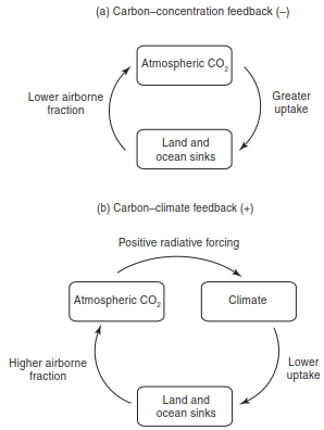
Fig. 29.12. Schematic representation of (a) the carbon–concentration feedback and (b) the carbon–climate feedback.

Mathematically, the total change in land carbon storage (ΔC_L, measured in Pg C) within this feedback framework is expressed as:

Where β_L (Pg C ppm⁻¹) represents the sensitivity of land carbon storage to atmospheric CO₂ concentration, γ_L (Pg C K⁻¹) denotes the sensitivity of land carbon storage to planetary temperature change, ΔC_A (ppm) is the change in atmospheric CO₂, and ΔT (K) is the change in global temperature. Analogous relationships apply to ocean carbon storage, defined by parameters ΔC_O, β_O, and γ_O.

Simulated Carbon Cycle Feedbacks. Experimental simulations by Cramer et al. (2001) comparing six global terrestrial biosphere models from 1861 to 2100 demonstrated that under CO₂-only forcing, CO₂ fertilization increased the land carbon sink to 1.4–3.8 Pg C yr⁻¹ in the 1990s (multi-model mean: 2.4 Pg C yr⁻¹) and 3.7–8.6 Pg C yr⁻¹ by 2100 (multi-model mean: 6.2 Pg C yr⁻¹). However, when climate change was included, climate-driven alterations in temperature and precipitation reduced the terrestrial sink to 0.6–3.0 Pg C yr⁻¹ in the 1990s (multi-model mean: 1.6 Pg C yr⁻¹) and 0.3–6.6 Pg C yr⁻¹ by 2100 (multi-model mean: 3.4 Pg C yr⁻¹). This reduction confirms a positive feedback loop between climate change and the carbon cycle (Friedlingstein et al. 2001).

To represent these feedbacks in climate projections, Earth system models (ESMs) integrate biogeochemical carbon cycles with physical climate processes, simulating transient climate conditions from 1850 to 2100 under prescribed atmospheric CO₂ concentrations or anthropogenic emissions.

Mechanisms of Terrestrial and Oceanic Carbon Processing. The terrestrial biosphere responds directly to elevated atmospheric CO₂ via photosynthetic enhancement (CO₂ fertilization), which acts as a negative feedback. Conversely, heterotrophic respiration increases with elevated soil temperatures, accelerating organic carbon decomposition and releasing CO₂ back into the atmosphere as a positive feedback. Climate change can enhance carbon uptake via increased net primary production (NPP) in cold or dry regions experiencing increased precipitation, but suppresses NPP in moisture-limited regions.

In ocean carbon cycle models, atmospheric CO₂ dissolves in seawater relative to its partial pressure. Oceanic carbon absorption is governed by physical and biological mechanisms:

· Temperature solubility: Carbon dioxide is more soluble in cold water than in warm water; warming sea surface temperatures reduce CO₂ solubility.

· Wind-driven exchange: Higher wind speeds increase air-sea gas exchange rates.

· Biological pump: Phytoplankton and zooplankton fix inorganic carbon into organic matter, which sinks to deep ocean sediments upon biological decay.

· Oceanic circulation: Vertical mixing and circulation patterns determine the transport rate of dissolved carbon from surface waters to deep ocean reservoirs.

Model Intercomparisons and Quantitative Feedback Metrics. The pioneering coupled carbon cycle-climate simulation by Cox et al. (2000) isolated carbon-climate feedbacks by comparing a biogeochemically coupled simulation (constant climate at CO₂ = 290 ppm) against a fully coupled simulation. In the fully coupled scenario, simulated atmospheric CO₂ reached approximately 980 ppm by 2100—about 250 ppm higher than in the uncoupled simulation. This amplifying feedback led terrestrial ecosystems to transition from carbon sinks to net carbon sources after the mid-twenty-first century, driven by soil carbon loss and Amazonian rainforest dieback under warmer, drier conditions.

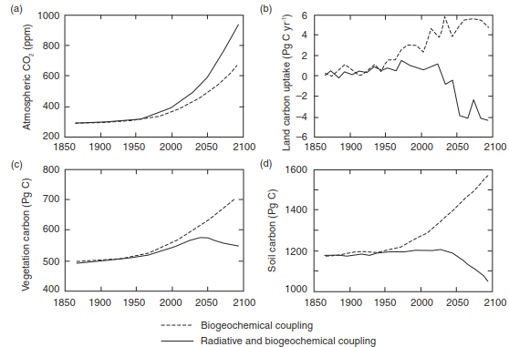
Fig. 29.13. Simulated (a) atmospheric CO₂ concentration, (b) global land carbon uptake, (c) global vegetation carbon, and (d) global soil carbon for 1860–2100 using the Hadley Centre HadCM3LC model with the TRIFFID dynamic global vegetation model. Shown are simulations with biogeochemical coupling (without carbon–climate feedback) and with radiative and biogeochemical coupling (with carbon–climate feedback). Adapted from Cox et al. (2004).

In a broader multi-model assessment, Friedlingstein et al. (2006) evaluated 11 ESMs for the IPCC Fourth Assessment Report (AR4). By 2100, oceanic carbon uptake ranged between 4–10 Pg C yr⁻¹, whereas terrestrial carbon flux exhibited wider variability, spanning from a 6 Pg C yr⁻¹ source to an 11 Pg C yr⁻¹ sink.

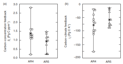
Fig. 29.14. Land carbon–concentration (a) and carbon–climate (b) feedback parameters for 11 models used in the Intergovernmental Panel on Climate Change (IPCC) fourth assessment report (AR4) (Friedlingstein et al. 2006) and 9 models used in the fifth assessment report (AR5) (Arora et al. 2013). Shown are the individual models (symbols) and the multi-model mean (star).

Across AR4 models, the land carbon-concentration feedback parameter (β_L) ranged from 0.2 to 2.8 Pg C ppm⁻¹ (mean: 1.4 Pg C ppm⁻¹), while the land carbon-climate feedback parameter (γ_L) ranged from -20 to -177 Pg C K⁻¹ (mean: -79 Pg C K⁻¹). In the IPCC Fifth Assessment Report (AR5, Arora et al. 2013), β_L averaged 0.9 Pg C ppm⁻¹ (range: 0.2–1.5 Pg C ppm⁻¹) and γ_L averaged -58 Pg C K⁻¹ (range: -16 to -89 Pg C K⁻¹). This represents a reduction in multi-model spread, partly due to model refinements.

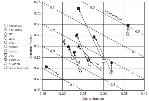
Fig. 29.15. Fraction of cumulative anthropogenic CO₂ emission in air, ocean, and land up to 2000 (open symbols) and to 2100 (closed symbols) for eleven Earth system models. Adapted from Denman et al. (2007).

All models confirm a declining capacity of land and ocean sinks to absorb anthropogenic CO₂ emissions over the twenty-first century, increasing the airborne fraction (Ballantyne et al. 2012; Le Quéré et al. 2013; Lombardozzi et al. 2014).

Regional Dynamics, Biogeochemical Constraints, and Emergent Constraints. Carbon cycle feedbacks display significant spatial heterogeneity. In warm tropical regions, increased evaporative demand can suppress NPP by drying soils, whereas high-latitude ecosystems often experience elevated NPP due to longer growing seasons and warming temperatures. Historically, CO₂ fertilization-induced terrestrial carbon accumulation is estimated to have reduced atmospheric CO₂ by 85 ppm, avoiding approximately 0.3°C of warming (Shevliakova et al. 2013).

A major source of uncertainty in carbon cycle projections involves nutrient limitation, particularly within the nitrogen cycle (Sokolov et al. 2008; Jain et al. 2009; Thornton et al. 2009; Zaehle et al. 2010a; Gerber et al. 2013). Models incorporating carbon-nitrogen (O-CN) interactions demonstrate that restricted nitrogen availability limits CO₂ fertilization responses, although accelerated nitrogen mineralization in warmer soils partially offsets this suppression.

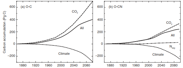
Fig. 29.16. Cumulative land carbon storage (1860–2100) in response to CO₂, climate change, nitrogen deposition (N_dep), and all forcings simulated by the O-CN terrestrial biosphere model. Simulations are for (a) carbon-only (O-C) and (b) carbon-nitrogen (O-CN) implementations of the model. Adapted from Zaehle et al. (2010a).

To constrain model uncertainties, researchers apply emergent constraints by linking short-term interannual variability in atmospheric CO₂ growth rates to long-term climate sensitivity (Cox et al. 2013; Wenzel et al. 2014). By constraining tropical land sensitivity (γ_LT) against observed tropical temperature anomalies (γ_IAV), Cox et al. (2013) revised estimated tropical land carbon release from an unconstrained 69 Pg C K⁻¹ down to 53 Pg C K⁻¹ (γ_LT = -53 Pg C K⁻¹), reducing the probability of extreme carbon loss (γ_LT < -100 Pg C K⁻¹) from 21% to 0.2%.

Atmospheric CO₂ Stabilization and Carbon-Climate Feedbacks

Atmospheric Stabilization and Mitigation Pathways. Stabilization of atmospheric CO₂ at a specified concentration in the future is a fundamental objective of global climate policy. Atmospheric carbon dioxide concentration represents a dynamic equilibrium between anthropogenic emissions (originating from fossil fuel combustion and land-use change) and carbon uptake by terrestrial biosphere and ocean carbon sinks. Quantifying allowable anthropogenic CO₂ emissions necessary to achieve target atmospheric concentration trajectories requires Earth system model simulations featuring an interactive carbon cycle (Ciais et al. 2013; Jones et al. 2013).

In emissions-driven simulations, fossil fuel emissions serve as prescribed inputs, while atmospheric CO₂ concentration (C_A) is calculated as a prognostic variable influenced by fossil fuel emissions (E_FF), land-use emissions (E_LU), the net atmosphere-land carbon flux (F_AL), and the atmosphere-ocean carbon flux (F_AO). The rate of change of atmospheric CO₂ over time is governed by the mass balance equation:

In concentration-driven simulations, atmospheric CO₂ trajectories are prescribed directly as input data. Land and ocean carbon pools respond to forced atmospheric CO₂ levels and consequential climate changes without dynamically altering the prescribed atmospheric concentration. In this framework, atmospheric concentration C_A is known, enabling the calculation of total compatible anthropogenic emissions (E_FF + E_LU) required to match the target profile based on modeled land and ocean fluxes:

Compatible Emissions Projections Across RCP Scenarios. Multi-model Earth system simulations demonstrate that total compatible fossil fuel emissions vary significantly across different Representative Concentration Pathways (RCPs) over the period 2012–2100 (Ciais et al. 2013):

· RCP 2.6: Multi-model mean compatible emission of 270 Pg C (multi-model range: 140–410 Pg C).

· RCP 4.5: Multi-model mean compatible emission of 780 Pg C (multi-model range: 595–1005 Pg C).

· RCP 6.0: Multi-model mean compatible emission of 1060 Pg C (multi-model range: 840–1250 Pg C).

· RCP 8.5: Multi-model mean compatible emission of 1685 Pg C (multi-model range: 1415–1910 Pg C).

Higher concentration pathways permit larger cumulative carbon emissions, but the precise allowable budget depends heavily on carbon cycle feedbacks. The positive carbon-climate feedback—wherein climate warming suppresses terrestrial carbon sink capacity—reduces ecosystem uptake of anthropogenic carbon, requiring further reductions in allowable emissions to meet stabilization targets (Jones et al. 2005, 2006; Matthews 2006). Conversely, the negative carbon-concentration feedback expands terrestrial carbon sequestration via CO₂ fertilization, allowing higher compatible emissions. However, nutrient limitations such as nitrogen or phosphorus availability constrain plant productivity enhancement, reducing the CO₂ fertilization effect and necessitating stricter emission limits to achieve stabilization goals.

Mechanistic Drivers and Uncertainties in Global Change Feedbacks. Feedbacks between the global carbon cycle, atmospheric CO₂ concentrations, and climate warming involve complex, interacting biogeochemical mechanisms, many of which remain underrepresented or absent in current model architectures. While the positive carbon-climate feedback is typically framed around temperature sensitivities of photosynthesis and respiration, models frequently neglect higher-order ecosystem responses such as extended growing season lengths, increased nutrient availability, shifting plant and microbial community structures, and altered water use efficiency (Luo 2007). Similarly, negative carbon-concentration feedbacks rely on simplified formulations of photosynthetic responses, while complex mechanisms regulating plant carbon allocation under elevated CO₂ remain inadequately understood (Norby and Zak 2011).

A major source of uncertainty stems from carbon-nitrogen biogeochemistry parameterizations. Earth system models vary widely in their representation of:

· Nitrogen availability constraints on photosynthesis and plant uptake.

· Stoichiometric C:N ratios in plant tissues and soil pools (whether fixed or dynamic).

· Gaseous nitrogen losses and biological nitrogen fixation rates.

· Plant-microbe competition for mineralized nitrogen (Zaehle and Dalmonech 2011).

· Secondary phosphorus limitations on plant growth and CO₂ responsiveness (Vitousek et al. 2010; Zhang et al. 2011, 2014; Goll et al. 2012; Yang et al. 2014).

Permafrost Degradation and Physiological Stress Dynamics. High-latitude permafrost soils store an estimated 1672 Pg of organic carbon. As Arctic temperatures increase, thawing permafrost exposes ancient organic matter to microbial decomposition, threatening substantial carbon releases to the atmosphere (Schuur et al. 2008, 2013). Nevertheless, the magnitude of the permafrost carbon-climate feedback remains poorly constrained due to uncertainties surrounding soil carbon decomposition rates following thaw, geographical mapping of permafrost distribution, and localized vulnerability to thermal degradation (Lawrence and Slater 2005; Koven et al. 2011, 2013; Burke et al. 2013; Slater and Lawrence 2013).

Plant physiological responses to severe heat and drought stress present additional modeling challenges. Most current models incorporate immediate enzymatic responses to temperature, but omit photosynthetic and respiratory thermal acclimation (Smith and Dukes 2013). Furthermore, key mechanisms governing drought-induced forest mortality—such as hydraulic failure and carbon starvation—are rarely represented (McDowell et al. 2008, 2013; McDowell and Sevanto 2010; Anderegg et al. 2012; Choat et al. 2012):

· Hydraulic failure: Occurs when water column continuity breaks within xylem conduits, forming gas embolisms (cavitation) under intense evaporative demand and low soil moisture. Cavitation disrupts xylem water transport, inducing rapid tissue dehydration.

· Carbon starvation: Initiated when stomata close to prevent water loss, which suppresses photosynthetic CO₂ assimilation while ongoing metabolic maintenance demands deplete internal carbohydrate reserves.

Demographic Processes and Terrestrial Ecosystem Regulation. Demographic drivers controlling community composition and succession are generally absent from standard biogeochemical models and present parameterization challenges for dynamic global vegetation models (DGVMs). Next-generation DGVMs incorporate structural advances in plant demography, ecosystem dynamics, and community organization (Fisher et al. 2010; Scheiter et al. 2013). However, simulating plant species migration in response to shifting climate zones remains problematic (Higgins and Harte 2006; Levis 2010).

Simultaneously, future land use and land-cover change configurations across twenty-first-century socioeconomic scenarios span a wide range of outcomes, from extensive global deforestation driven by agricultural expansion to widespread regional reforestation following agricultural abandonment (Brovkin et al. 2013). Although Earth system models represent simplified abstractions of interconnected physical, chemical, biological, and human systems, the emerging scientific consensus highlights terrestrial ecosystems as a central regulator of the global carbon cycle and climate system.