Net Ecosystem Production and Net Biome Production

Integrating over all assimilatory and respiratory processes taking place at the same time in a terrestrial ecosystem becomes necessary if one is interested in the response of ecosystems to management or climate or if one wants to compare flux magnitudes across ecosystem types. Measuring all processes separately and scaling them up to the ecosystem level is impossible and would introduce a huge uncertainty into the final flux estimate (Sect. 14.1, Chap. 14). Thus, one uses a micrometeorological approach (eddy covariance method, Box 16.1) to directly measure net carbon dioxide fluxes between the ecosystem and the atmosphere, that is, the net ecosystem CO₂ exchange (NEE) (in pmol CO₂ m^-2 s^-1).

NEE data are typically given using the meteorological sign convention (from an atmospheric perspective): negative values represent situations where the atmosphere loses CO2 while the ecosystem takes up CO2 and acts as carbon sink; positive values represent situations where the atmosphere gains CO2 while the ecosystem loses CO2 and acts as a carbon source. NEE is measured continuously over long time periods at high temporal resolution, typically at 10-20 Hz (10-20 times per second). The longest time series reaches back to 1992 (Harvard Forest, USA), and today data from >850 flux tower sites are available globally (Sect. 14.1, Chap. 14).

Summing up NEE (generally aggregated to 30 min averages) to annual values results in net ecosystem production NEP (typically in g C m^-2 year^-1), which is given as a positive number to represent a carbon sink (in contrast to NEE!). NEP is the small net difference between two large fluxes, GPP and all auto- and heterotrophic respiratory losses (Eq. 16.17), and can be approximated by NPP minus heterotrophic respiration. When no additional C inputs such as fertilisation and no additional C exports such as harvests, fire or erosion occur, NEP represents the ecosystem carbon budget, that is, the ecosystem C sink or source. However, when additional inputs and exports occur, these C fluxes need to be taken into account when calculating the ecosystem carbon budget.

Then the C budget is called net biome production (NBP) (Eq. 16.18) (Schulze et al. 2000), even if a field or ecosystem type (and not a biome) is studied:

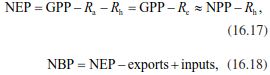
where R_a is the respiration of autotrophic plants, R_h the respiration of heterotrophic organisms, and R_e the total ecosystem respiration, with R_e = R_a + R_h. Exports are additional C losses and can be harvests, C emitted as BVOCs, fire or erosion. Inputs are additional C sources such as organic fertilisers, that is, slurry and manure.

Most of the carbon enters the ecosystem as CO₂ via GPP (except organic fertilisation; see subsequent discussion). About 50% of GPP is used for NPP (Fig. 16.17). The NPP/GPP ratio, also called carbon use efficiency, varies with vegetation type and responds to changes in environmental conditions. Median values of NPP/GPP, considering ANPP and BNPP, range from about 0.3 for boreal forests, to 0.4 for temperate coniferous, 0.5 for tropical forests and 0.55 for temperate deciduous forests (DeLucia et al. 2007). Using remote sensing, the ANPP/GPP ratios can be estimated (Zhao et al. 2005), resulting in values between 0.35 and 0.54 for forests, 0.58 for cropland and 0.65 for grasslands, validated by inventories and flux measurements.

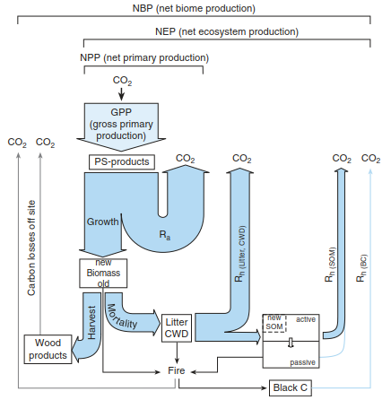
Fig. 16.17. Carbon budget of forest ecosystems. The initial process is gross primary production (GPP), which corresponds to gross photosynthesis. About 50% of the photoassimilates are used for net primary production (NPP); the rest is available for growth respiration and maintenance respiration. Accounting for heterotrophic respiration from litter, coarse woody debris (CWD) and from soils leads to net ecosystem production (NEP). If further processes are considered that remove or add C from or to the system, one talks about net biome production (NBP). CWD coarse woody debris, SOM soil organic matter, BC black carbon, Rh heterotrophic respiration, Ra respiration of autotrophic plants (After Schulze et al. (2000)

To know when an ecosystem is a carbon sink or a source, the net balance between gross photosynthesis and ecosystem respiration needs to be known. The diurnal courses of NEE clearly show when a particular process dominates. During the night, only respiration occurs. During the day, photosynthesis can be compensated by respiration (often the case in winter) or photosynthesis can overcompensate respiration (during most of the growing season). Thus, depending on the time of day and the day of the year, the ecosystem acts as either a CO2 source (nighttime, winter) or a CO2 sink (daytime, growing seasons). This general pattern occurs throughout the year, but environmental conditions, phenology and management determine the relationship of CO₂ loss to uptake and, thus, the daily NEE flux.

The NEE of an intensively managed temperate grassland shows photosynthetic activities already in spring and highest uptake during summer (green and blue colours in Fig. 16.18a) (Zeeman et al. 2010). Therefore, sink activities start as early as February/March if the winter is mild (as in winter 2006/2007) but can also be delayed until April/May (as in winter 2005/2006). During the main growing season (May to September), high CO2 uptake rates are measured during the day and only interrupted by management interventions, that is, frequent cuts of the meadow and subsequent manure applications. Then photosynthesis drops to very low rates and respiration dominates, both from the soil and the manure (orange and red colours in Fig. 16.18a).

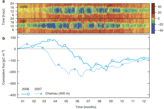Fig. 16.18. Annual and diel courses of net ecosystem CO₂ exchange of an intensively managed grassland over 2 years. Net ecosystem CO₂ fluxes in pmol CO₂ m^-2 s^-1 were measured with the eddy-covariance method at Chamau, Switzerland, located 400 m asl. a Net ecosystem CO2 fluxes are given in the micrometeorological sign con vention over 24 h for the 2 years 2006-2007. b Seasonal courses of cumulative CO₂ fluxes differ between the 2 years. Frequent grass cuts (6-7 per year) and subsequent manure applications result in the typical zigzag pattern of CO₂ fluxes in grassland. (Data from M. J. Zeeman)

Presenting the cumulative NEE fluxes (Fig. 16.18b) reveals a typical zigzag pattern over the course of the growing season. When the grassland has grown well (NEE very negative, indicating high CO2 uptake; data at the lowest point in a zigzag pattern), the farmer will cut the meadow to harvest the biomass and subsequently apply manure to fertilise the vegetation. Thus, after the harvest, photosynthesis is small and soil respiration dominates NEE for some days (NEE becomes less negative; data on the upward-pointing leg of a zigzag). When the regenerating vegetation carries out enough photosynthesis to overcompensate soil respiration, NEE will become more negative again (data on the downward-pointing leg of a zigzag). This zigzag pattern will repeat itself with each combined cut-and-manure event. At the end of the year, this grassland shows a carbon balance between assimilation and respiration of about 90 g C m^-2 year^-1 (Fig. 16.18b). However, this balance is not yet the ecosystem carbon budget since the grassland was harvested multiple times (C exports) and received large amounts of organic fertiliser (C inputs). Accounting for the carbon in these additional exports (about 350 g C m^-2 year^-1) and inputs (about 330 g C m^-2 year^-1), the NBP and, thus, the ecosystem carbon sink was about 70 g C m^-2 year^-1.

If an ecosystem does not experience additional exports and inputs during the year (e.g. by management or DOC fluxes), the final value of the cumulative NEE curve gives an estimate of the ecosystem carbon sink. This is often the case in forests, which are not managed on an annual basis. Evergreen forests can exhibit small sink activities also over winter, while sink activities in deciduous forests start with the leaf-out of the understorey vegetation (e.g. Allium ursinum, wild garlic, in temperate beech forests) and show peak NEE fluxes when the tree canopy is fully developed. Thus, phenology is an important driver of NEE and NEP. The longer the growing season, the higher the NEP: deciduous broadleaf forests increase their NEP by 5.6-5.8 g C m^-2 per day of the growing season, evergreen needle-leaf forests by 3.4 g C m^-2 day^-1, savannas by 3.7 g C m^-2 day^-1 and grasslands and croplands by 7.9 C m^-2 day^-1 (Churkina et al. 2005). Climate variables have large effects on NEE, but also on GPP and R_e. Both component fluxes depend primarily on light but increase with temperature and precipitation until limitations set in (heat or freezing stress, drought).

This is true not only of the current year’s weather but also of the previous year’s weather, since carbon allocation and storage drive bud establishment and growth the following year. Furthermore, disturbances, either slow or sudden, affect ecosystem CO₂ fluxes. N deposition was shown to increase the NEP. Fire frequency and intensity affect both GPP and R_e. Drought and heatwaves affect GPP more negatively than R_e, shifting ecosystem NEE towards respiratory losses and even releasing CO₂ from SOM, sometimes worth several years of C sequestration (Ciais et al. 2005). Old forests still sequester carbon (Sect. 14.1, Chap. 14), although sometimes at lower rates than mature forests. For further examples, please see Baldocchi (2008, 2014).

Net ecosystem CO2 fluxes, that is, the very small net difference between GPP and Re, are measured using a micrometeorological approach (Table 16.5). However, these two very large component fluxes can be estimated using so-called partitioning techniques (e.g. Reichstein et al. 2005). Partitioning is typically based on the relationship of nighttime NEE (R_e only) to temperature, using relatively short time windows (often about 2 weeks). GPP is then calculated as the difference between NEE and Re, assuming that leaf respiration during the day does not differ significantly from leaf respiration at night. Site-specific adjustments to this simple partitioning routine might be necessary, for example, when the site has been managed or a disturbance has occurred (fire, disease, extreme event). NEP is highest for forests (except boreal) and lowest for desert ecosystems (but data availability is very limited) (Table 16.5). Uncertainties are typically between 10 and 30% or between 30 and 50 g C m^-2 year^-1.

This uncertainty corresponds to about half the weight of normal printer paper (with about 80 g m^-2) covering 1 m² of ground (Baldocchi 2008). GPP and Re estimates are much larger than NEP but follow the same patterns across ecosystem types. Fluxes of agricultural ecosystems, that is, grasslands and croplands, are comparable to those of temperate forests. While more than 850 site- years are available for NEE measurements and, thus, GPP and Re estimates, not many NBP estimates exist, so uncertainties are very large.

Those given in Table 16.5 rely on a combination of measurements and models. The NBP/NPP ratio can be used as a proxy for the carbon sequestration efficiency. It is reported to be 0.15 ± 0.05 for forests, 0.13 for grasslands and varies between -0.03 and 0.01 for croplands (Ciais et al. 2010; Luyssaert et al. 2010). These estimates support the more robust patterns based on NEP measurements, with forests being the largest carbon sinks, grasslands being small carbon sinks, and croplands being not carbon sinks at all but rather carbon sources.

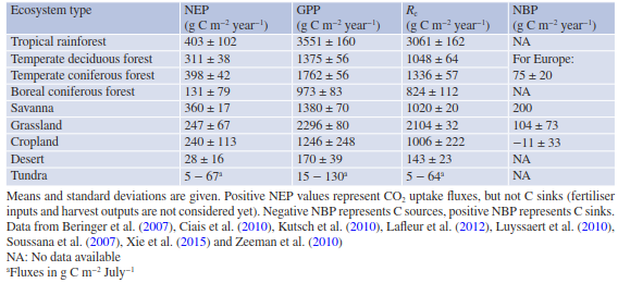
Table 16.5. NEP, GPP, R_c and NBP estimates across ecosystem types

The long-term development of the terrestrial carbon sink for any given ecosystem will depend on the fraction of how much carbon enters these sinks (e.g. expressed as NBP/NPP) and the longevity or MRT of the carbon sequestered in these sinks. Both main sinks in ecosystems, wood and SOM, have MRTs that can be up to several decades (tropical, temperate climate) to centuries (boreal, arctic climate), but only very small amounts of C enter these long-term sinks. Integrating over all vegetation and soil carbon stocks, global ecosystem MRT has been calculated as 22.5 years, ranging from 18.1 to 29.4 years (Table 16.6) (Carvalhais et al. 2014). Thus, the longevity of global carbon sinks is rather short and thus sensitive to environmental change. The longest MRTs are found in tundra and boreal forests, while the shortest MRTs are found in tropical forests and savannas. Averaging all MRT > 75°N results in a MRT of 255 years, compared to 15 years in the equatorial tropics. Ecosystem MRTs vary with annual air temperature and annual precipitation, and climatic variables are predicted to change in the future (Chap. 23).

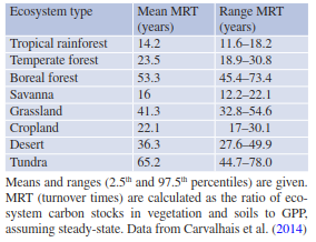
Table 16.6. Mean residence times of entire ecosystems

Stable carbon isotopes as well as radiocarbon (Sect. 16.2.1) data provide further insights into the carbon turnover and the fate of carbon within an ecosystem. The source of carbon dioxide for plant photosynthesis is atmospheric CO2, which currently has a δ¹³C value of about -8.3%c (declining due to fossil fuel burning; Sect. 23.3 in Chap. 23). Within the canopy, atmospheric CO₂ is mixed with respired CO₂, which has a δ¹³C value close to the organic substrate being respired (between -30 and -18%e for C₃ plants), resulting in canopy δ¹³C profiles between the atmospheric background at the top of the canopy (Fig. 16.19) and a mix of both CO₂ sources close to the ground (reaching values of around -14 to -16%e). δ¹³C gradients in canopy CO2 vary with time of day, being small during the day when turbulent mixing occurs within the canopy and large at night under stable atmospheric conditions.

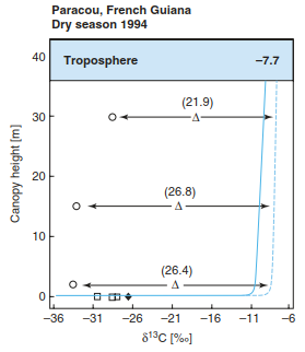
Fig. 16.19. Conceptual model of stable carbon isotope ratios δ¹³C and leaf carbon isotope discrimination A (in per mil compared to an international standard) in a tropical forest in French Guiana. Foliage values (circles) are given for different heights within the canopy. Soil and Litter (squares) and soil-respired CO₂ (diamond) signatures are given. Canopy CO₂ values (lines) are given for night- (solid) and daytime (dashed). (Buchmann et al. 1997)

This canopy CO2 with its δ¹³C is then the source for photosynthesis. Discrimination against ¹³CO2 happens during CO2 diffusion into foliage as well as during CO2 fixation (and respiration) (for detailed reviews see Ghashghaie and Badeck 2014 and Werner and Gessler 2011). Thus, depending on where the foliage is located within a canopy, not only the ecophysiology of foliage but also the source δ¹³C determines the foliar δ¹³C values in any ecosystem. As a result, foliage in the top canopy has higher δ¹³C values than foliage closer to the ground (Fig. 16.19). In general, 30% of the gradients in foliar δ¹³C are due to canopy CO2, about 70% to ecophysiology. If foliage senesces and becomes litter and SOM, δ¹³C values increase owing to fractionation during mineralisation and processes related to decomposition. Similarly, soil-respired CO2 has a higher δ¹³C than SOM. For further details, please refer to Bruggemann et al. (2011).

Moreover, the δ¹³C in foliage integrates over the entire lifespan of a leaf, while δ¹³C litter integrates over all species currently present in an ecosystem. In turn, δ¹³C of SOM integrates over current and past vegetation. This is particularly interesting when vegetation had changed from C₃ to C₄ vegetation or vice versa, since carbon isotope discrimination differs strongly between these two photosynthesis types (Sect. 12.2, Chap. 12). Thus, δ¹³C of SOM within a soil profile can give information about the dominant vegetation, forest or (C₄) grassland, over time, particularly when the age of SOM is known. The difference between the δ¹³C of atmospheric CO₂ entering the ecosystem for GPP and the δ¹³C of respired CO₂ of ecosystems, the so-called isotopic disequilibrium, is an important piece of information for global inverse atmospheric models that are used to estimate global sinks and sources.

Fluxes of CH₄ and Other Biogenic Volatile Organic Compounds

Although CO2 dominates the discussion about the carbon dynamics of ecosystems, CO2 is not the only carbon-containing gas being exchanged between ecosystems and the atmosphere: the exchange of methane (CH₄) and other BVOCs are highly relevant for many ecosystems as well.

Biogenic methane is produced by bacteria (Archaea; methanogenic bacteria) in anaerobic zones in soils and is a potent greenhouse gas (Fig. 16.20) (Chap. 23). The highest CH₄ production is thus found in wet or waterlogged soils, for example, in rice paddies and wetlands. However, between 60 and 90% of the CH₄ produced is oxidised to CO2 by methanotrophs, that is, bacteria widespread in soils, representing a large sink for CH4, which is relevant for global change (Le Mer and Roger 2001). CH₄ emissions from soils to the atmosphere can happen via diffusion or as bubbles from wetland soils (called ebullition), but also via vascular plants.

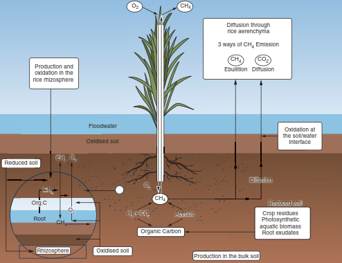
Fig. 16.20. CH₄ emissions from soils, mediated by vascular plants (Le Mer and Roger 2001)

Here, the aerenchyma of wetland plants (such as Carex species or Eriophorum vaginatum) acts like a chimney for CH4, bypassing potential oxidation in the upper soil layers, thereby increasing CH4 emissions from these ecosystems. The aerenchyma of aquatic or wetland plants (mainly in herbaceous plants but also in Alnus) is a modified parenchyma tissue with large cavities formed under anoxic conditions to mediate gas exchange (mainly of oxygen) between shoots and roots. Outgassing of CH₄ via aerenchyma tissues can be responsible for up to 90% of the CH4 emissions during the growing season. The chimney effect increases with higher soil carbon contents, is higher under convective than under stable atmospheric conditions, and has been reported to scale with stomatal conductance (Joabsson et al. 1999; Le Mer and Roger 2001).

Plants emit a wide range of BVOCs such as isoprene (C₅H₈) and methanol (CH₃OH), the two most abundant BVOCs after CH4 (Guenther et al. 2012), but up to 1700 substances have been reported (Loreto and Schnitzler 2010). Plants use BVOCs to communicate with each other, but also with other organisms, for example, as a wound signal (Sect. 19.3 in Chap. 19), and constitute up to 2-5% of the net carbon gain of heavily emitting broadleaf trees (e.g. Eucalyptus, Quercus and Populus). But BVOCs have also been found to relieve oxidative and thermal stresses. Two environmental factors typically increase foliar BVOC emissions, temperature and light, while water stress does not show an effect. While many of these flux measurements were made using small leaf enclosures (Guenther et al. 2012), such fluxes have also been measured at the ecosystem level using micrometeo- rological techniques (Sect. 14.1 in Chap. 14) (Wohlfahrt et al. 2015).

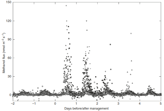
Fig. 16.21. Methanol emissions from three temperate grasslands in Austria and Switzerland measured using micrometeorological techniques. Large peaks can be seen 1–3 days after the corresponding management events. Different symbols depict different sites. (Wohlfahrt et al. 2015)

Although these measurements supported environmental and biological controls, they also provided clear new evidence that, for example, ethanol fluxes are bi-directional: into and out of terrestrial ecosystems. In addition, land-use practices, such as clearing of understorey vegetation in forests or cutting of meadows with subsequent manure application, increased methanol emissions significantly over a couple of days (Fig. 16.21). Under a future climate, BVOC emissions are expected to increase owing to global warming, with large effects on atmospheric chemistry (Penuelas and Staudt 2010).