Phylogenetic Diversity. Environmental Controls of Biodiversity

Next to the use of functional, trait-based indices, the quantification of phylogenetic diversity is the second approach to measuring biodiversity based on species ecological differences. The concept relies on the simple assumption that the more time that has passed since two species shared a common ancestor, the higher the probability that they have ecologically and functionally diverged. Thus, this measure of biodiversity takes evolutionary history into account. For the calculation of phylogenetic diversity, the phylogenetic trees of the organisms occurring in a community must exist, and phylogenies of many different taxa have become increasingly available in recent decades owing predominantly to genomesequencing efforts.

In principle, community phylogenetic diversity is then calculated as the sum of the phylogenetic branch lengths connecting all taxa in a community and is thus a measure of the total amount of phylogenetic distance or evolutionary divergence in a community (Fig. 20.10). Because traits are the product of evolution, phylogenetic diversity encapsulates the entire evolved trait space of a community. In consequence, it can thus be used as a surrogate for trait diversity, for example, in cases where trait information is limited (Cadotte et al. 2010).

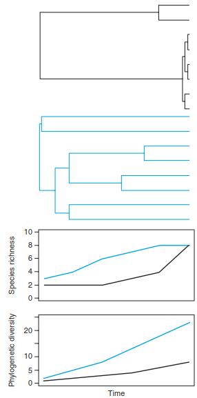
Fig. 20.10. Development of species richness and phylogenetic diversity through time. The black phylogeny represents a community or region with recent speciation events, and the blue phylogeny represents a situation with older speciation events. Both phylogenies ultimately produce the same number of species, but the accumulated branch lengths (i.e. phylogenetic diversity) in the blue phylogeny is much higher because of early diversification (Swenson 2011). Reproduced with permission from the Botanical Society of America

Phylogenetic diversity is an important aspect in studying the evolutionary processes that produce patterns of biodiversity and to understand the ecological interactions that determine species assemblage (Sect. 20.3). Being a surrogate of the functional structure of communities, it is also used to test hypotheses about the relationship between plant diversity and ecosystem functioning (Sect. 20.4). In addition, it is an important measure to define conservation priorities because communities with a high phylogenetic diversity.

Environmental Controls of Biodiversity.Plant species have evolved in certain areas and are adapted to specific environmental conditions. Hence, they are not evenly distributed across the globe or within their range. There are hostile regions, such as high alpine summits or extreme deserts, but also favourable regions, such as tropical rain forests. In consequence, plant diversity shows striking spatial patterns at various spatial scales, that is, at the global level (Fig. 20.11), but also within regions, landscapes or sites. Describing and understanding the causes of such differences in species distribution and diversity (biogeography) has a long tradition, with Alexander von Humboldt being the first to analyse the environmental constraints of plant distribution (von Humboldt 1808), followed by the seminal work of Andreas Franz Wilhelm Schimper (1898).

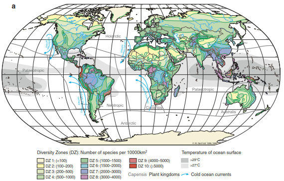
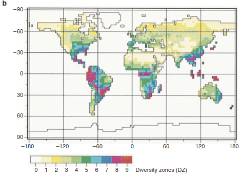
Fig. 20.11. Maps of global plant species richness. a Species richness based on empirical data from inventories and data on abiotic factors, including climate. The diversity zones (DZs) are grouped according to species numbers per 10,000 km2 (Barthlott et al. 2005). Reproduced with permission from the Deutsche Akademie der Naturforscher Leopoldina - Nationale Akademie der Wissenschaften. b Species richness derived from simulations based on growth-limiting climatic scenarios only. The values are categorised into nine groups: (1) <2%, (2) 2–4%, (3) 4–10%, (4) 10–20%, (5) 20–30%, (6) 30–40%, (7) 40–60%, (8) 60–80%, and (9) 80% of the maximum diversity value simulated. (Kleidon and Mooney 2000)

In the preface of his book, Schimper wrote (the following quotes are taken from the authorised English translation by W. R. Fisher: Schimper 1903): “The delimitation of separate floral districts and their grouping into more comprehensive combinations are nearly completed, and the time is not far distant when all species of plants and their geographical distribution will be well known. The objectives of geographical botany will not, however, then be attained, as is often assumed, but a foundation merely will have been laid on which science can construct a larger edifice.

The essential aim of geographical botany will then be an inquiry into the causes of differences existing among the various floras” (p. v). Further, he already acknowledged the intimate connections between natural history and experimental sciences needed to disentangle the underlying causes of biodiversity patterns: “The oecology of plant distribution will succeed in opening out new paths on condition only that it leans closely on experimental physiology, for it presupposes an accurate knowledge of the conditions of the life of plants which experiment alone can bestow” (p. vi).

The following sections mainly describe patterns of plant species richness across environmental gradients and their underlying mechanisms. Clearly, biodiversity today is greatly changed by humans, for example, through land-use change and management, eutrophication or, increasingly, also by climate change. These aspects are described in more detail in Part V.