Continuous Indices of Functional Diversity

Much information is lost by any classification procedure because many traits are not categorical but continuous and plastic. In addition, using functional groups implies that species within those groups might be exchangeable or redundant when it comes to determining the effects of diversity on ecosystems (Sect. 20.4). Continuous measures of functional diversity, in contrast, capture the heterogeneity and variability of traits within a community. These measures can be calculated for single traits (e.g. asking the question whether the variability of leaf N concentration can better explain primary production than its mean value) or for multiple traits together (e.g. whether a higher or lower variability of leaf N concentration, cuticula thickness and LDMC better explains herbivory rates).

More than a dozen such continuous indices of functional diversity have been suggested that are based on slightly different assumptions and mathematical approaches. There are guidelines on how to select the most suitable index for specific questions (Schleuter et al. 2010; Petchey et al. 2009), and software solutions are available to calculate them (e.g. several online R scripts, FDiversity) (Pla et al. 2012). In principle, these indices can be divided into three groups that represent different aspects of functional diversity: functional richness, functional evenness and functional divergence (Fig. 20.9) (Mason et al. 2005). The first two are derived from indices to describe taxonomic diversity (Box 20.1). The latter two indices may also contain information about species’ abundances by weighting the contribution of each species based on cover or biomass, for example.

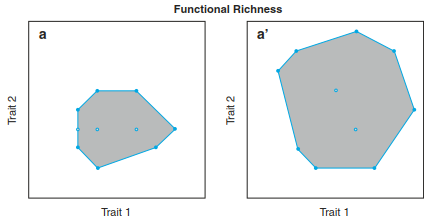
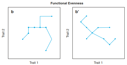
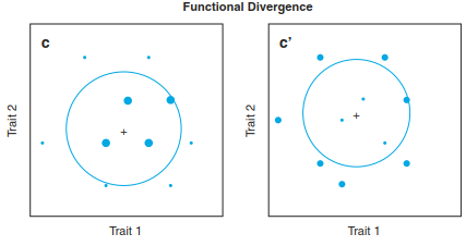
Fig. 20.9. Geometrical presentation of functional diversity indices. Two traits define a two-dimensional functional space for a local community of ten species (dots). Species are plotted in this space according to their respective trait values, with symbol size proportional to their abundances. The functional diversity of a community is thus the distribution of species and of their abundances in this functional space. For each component of functional diversity, two contrasting communities are represented, with low a, b, c and high a′, b′, c′ index values. Functional richness a and a′ is the functional space occupied by the community, functional evenness b and b′ is the regularity in the distribution of species abundances in the functional space, and functional divergence c and c′ quantifies how species abundances diverge from the centre of the functional space

Functional richness represents the volume of the functional trait space that is occupied by the species present in a community (Fig. 20.9a, a'). It therefore reflects the potentially used niche space by a community, that is, the hypervolume of a Hutchinsonian multidimensional niche. It can be used to test the hypothesis whether ecosystem properties depend on the size of the functional space covered. For example, it could be hypothesised that a community composed of species with very different rooting depths and plant heights (i.e. high functional richness) can take up more nutrients from the entire soil profile and capture more light, and hence produce more biomass, than a community composed of flat rooting species and small statured plants only (Fig. 20.38). The index is positively correlated with species richness, but communities with the same number of species may differ in functional richness if the traits are more similar in one community than in others.

Functional evenness measures the regularity in the distribution of species abundances in the occupied trait space, with high values representing a rather regular distribution of traits (Fig. 20.9b, b'). Functional evenness can also be linked to the utilisation of resources. Staying with the aforementioned example, it could be tested whether a community with an even distribution of rooting depths and plant heights (i.e. high functional evenness) is more productive than a community dominated by flat rooting small plants because the soil profile and the above-ground space are more evenly occupied and utilised, which could lead to higher nutrient uptake and light capture.

Functional divergence estimates the position of species within the trait space, for example, by quantifying how species abundances diverge from the centre of the functional space (Fig. 20.9c, c'). A high value means that very abundant species are very far from the centre of the trait space. In our example, it can be tested whether communities with large differences in rooting depths and heights (i.e. high functional divergence) may have a high degree of niche differentiation and low competition for resources (Sect. 20.4.9), potentially resulting in increased productivity, in comparison with communities dominated by species with small differences in these two traits.