Environmental Heterogeneity and Species Diversity

The relation between environmental heterogeneity and species richness, as mentioned earlier in connection with alpine regions, has for a long time attracted many ecologists in the search for mechanisms driving gradients in species diversity. Almost 100 years ago, Thienemann (1920) formulated two “biocoenotic laws” stating that the more diverse the environmental conditions and the closer they correspond to the “biological optimum”, the larger the number of species, and vice versa. It has been argued that spatial environmental heterogeneity could promote species richness through three major mechanisms (Stein et al. 2014). The first mechanism is based on classical niche theory (Sect. 19.3): the available niche space (in a Hutchinsonian sense, defined as an я-dimensional hypervolume, with the dimensions being environmental conditions, resources and biotic factors) should become larger if environmental gradients become steeper, if the amount of habitat types and the number of resources available increases, or if the physical structure of habitats becomes more complex. More species can be packed into a larger niche space.

The second mechanism is related to the ability of species to persist against adverse conditions: environmentally heterogeneous areas should provide more possibilities for shelter and refuge. This has nicely been demonstrated in topographically highly structured alpine communities. Temperature variability on the same slope of alpine grassland varies substantially at very short distances. Plant species adapted to cool habitats, with low indicator values for temperature, grow in significantly colder micro-habitats than plants with higher indicator values found on the same slope (Fig. 20.13). Thus, species may find suitable conditions matching their thermal niche within short distances to compensate for climate warming.

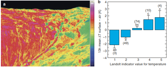
Fig. 20.13. Small-scale temperature heterogeneity in alpine grasslands. a False colour image based on infrared thermography of surface temperatures on a NNW exposed slope at the Furka Pass in the Swiss Alps under full direct solar radiation (12–18 h, August). Dark blue represents cold (2 °C) and magenta hot (24 °C) surface temperature (Scherrer and Körner 2010). Reproduced with permission from John Wiley & Sons. b Seasonal temperature differences between surface and air temperature during daytime hours per group of temperature indicator values. The numbers in brackets indicate the number of plant species within the different indicator groups; significant differences are denoted by different letters

As a third mechanism, evolutionary processes leading to diversification are accounted for: opportunities for isolation and divergent adaptation to diverse environmental conditions should increase with increasing environmental heterogeneity, resulting in a higher probability of specia- tion events. A number of studies have tested these different mechanisms and found general support of the heterogeneity-diversity hypothesis, though generalisations are difficult owing to the different research approaches, terminology and spatial scales studied. Recently, a worldwide metaanalysis that used data from 190 independent studies found general support for the environmental heterogeneity hypothesis (Stein et al. 2014). Different measures of environmental heterogeneity, including those related to land cover, vegetation diversity and structure, climate, soil variables and topography, were all positively related to species richness of plants, invertebrates and vertebrates (Fig. 20.14).

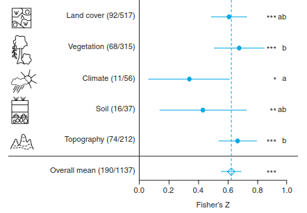
Fig. 20.14. Positive relationship between environmental heterogeneity and species richness. Effects of environmental heterogeneity were analysed separately for different categories (land cover, vegetation, climate, soil, topography). Mean effect sizes (Fisher’s z) that are significantly larger than zero indicate positive relationships; lines show 95% confidence intervals. Different letters indicate significant differences among categories. Diamond and dashed lines represent the overall weighted mean effect. Numbers in parentheses give the respective numbers of studies/data points. All coefficients are different from zero at significance levels: ***p < 0.001, **p < 0.01, *p < 0.05. Modified from Stein et al. (2014)

Closely related to the heterogeneity-diversity hypothesis is the intermediate disturbance hypothesis (Huston 1979), which postulates that the highest species richness will be found at intermediate levels of disturbance: at very low levels of disturbance, competitive species dominate the community and diversity is low (competitive exclusion); increasing levels of disturbance intensity or frequency may result in a disproportional mortality of the dominant species and larger environmental heterogeneity, resulting in postponed competitive exclusion, coexistence and, thus, higher diversity; very intensive disturbance events may lead to a failure of populations to recover from mortality and to a homogenisation of environmental conditions (Sects. 13.5 and 17.3).

Thus, there should be a trade-off between the ability of a species to compete with others and their ability to tolerate disturbance. Despite being a well-recognised hypothesis, the literature shows a variety of disturbance-diversity patterns, not a consistent peak as predicted by the intermediate disturbance hypothesis (Mackey and Currie 2001). Nevertheless, disturbance is an essential feature for ecosystem dynamics and affects biodiversity to a large degree. It is a natural component in all ecosystems, working at different spatial and temporal scales. For example, soil disturbance by ants or moles creates sites free of competitors for the germination and growth of seedlings; strong crown fires eliminate dominant tree species, reducing competition for light and soil resources and allowing the establishment of other species (Fig. 20.15); ground fires destroy thick layers of litter that otherwise cannot be penetrated by seedlings and increase mineralisation of litter- sequestered nutrients (Sect. 13.5). If such disturbances additionally act as barriers between populations, mutations that may lead to new species will have a better chance of getting established, leading to diversification over time (Sect. 17.2), as in the Mediterranean flora of the South African Cape region or the tropical Andes, for example.

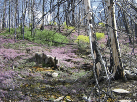
Fig. 20.15. Disturbances create “windows of opportunities” for species establishment. Species previously absent from a plant community are able to colonise a site after disturbances, such as fire. Saponaria ocymoides (pink flowers) and Isatis tinctoria (yellow) 4 years after a stand-replacing fire in the Swiss Alps (Leuk)

In the examples presented in the previous sections, plant diversity is statistically treated as the response variable, while abiotic and biotic site factors (e.g. availability of light, water and nutrients; disturbance regimes; herbivory) or modulators (e.g. temperature, pH) represent the independent variables that determine or explain the distribution of plant species and their diversity (Fig. 20.1). In the following section, we want to present in more detail one example of such biodiversity research, which is important to understand when we later discuss the functional importance of plant diversity (Sect. 20.4).