Productivity—Species Richness Relationships

There are striking biogeographical patterns of plant species diversity and several hypotheses exist to explain those patterns (Sect. 20.3.1). According to the energy-diversity hypothesis, plant diversity correlates well with measures of productivity along latitudinal gradients. Is this relationship ubiquitous and observable at various spatial scales?

Indeed, several studies have found relationships between some measures of productivity and plant species richness. It must be noted that productivity, defined as the net flux of carbon from the atmosphere into green plants per unit area and time (e.g. g m^-2 year^-1) is difficult to measure directly in the field (Sects. 12.5 and 14.1). Instead, often indirect measures that correlate to varying degrees with the potential or actual productivity of a site are used, such as actual evapotranspiration (Sects. 10.1 and 16.1), rainfall, peak above-ground biomass or annual biomass production. For example, in the Mongolian steppe biome, Bai et al. (2007) observed a positive linear relationship between above-ground biomass and plant species richness at various spatial scales and grazing intensities (Fig. 20.16).

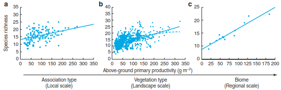
Fig. 20.16. Positive linear relationship between above-ground primary productivity and plant species richness. This example comes from the Inner Mongolia region of the Eurasian steppe and shows the productivity–diversity relationship across different spatial scales, a at the level of the plant community (Stipa grandis association), b at the level of the vegetation type (typical steppe), and c at the level of the entire biome (by association type). The fitted lines represent statistically significant linear (solid line) and quadratic (dashed line) relationships between productivity and species richness (Bai et al. 2007)

However, other empirical studies reported unimodal or hump-shaped relationships (also referred to as humped-back model), with a peak of species richness at intermediate productivity levels and a decrease at very low or high productivity (Fig. 20.17). Such a decrease at high productivity—usually associated with high nutrient availability (Sect. 11.1)—was observed in natural situations or with modified levels of productivity, for example, through fertilisation. A famous example of reduction in plant species diversity by increasing nutrient levels and associated productivity comes from the Park Grass Experiment in Rothamsted, England, where grassland plots have been treated with different fertilisers since 1859.

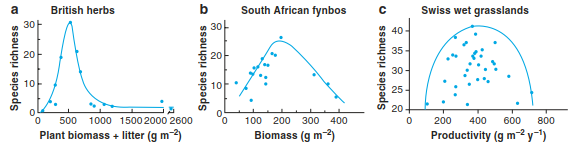
Fig. 20.17. Examples of hump-shaped relationship between productivity and plant species richness: a in British herb-dominated communities (Al-Mufti et al. 1977). Reproduced with permission from Blackwell Publishing Ltd.; b in South African Fynbos communities (Bond 1983); c in pre-alpine wet grasslands in Switzerland (Schmid 2002)

This decrease of diversity has been compared with the paradox of enrichment of predator-prey models (i.e. that increasing availability of resources may destabilise populations, which eventually can crash) (Rosenzweig 1971). Eutrophication, via high input of fertilisers or atmospheric deposition, therefore usually leads to severe declines in plant diversity (Sect. 23.5).

b South African fynbos

What could be the underlying mechanisms producing a hump-backed productivity-diversity relationship? Several different, not mutually exclusive, mechanisms have been proposed for the increasing and decreasing part of the hump and for the peak (Fig. 20.18). In short, the hump may be the result of varying levels of resource availability and heterogeneity and of disturbance (Grime 2001). Low productivity is a result of low resource availability, as well as of low resource heterogeneity and high disturbance. These conditions allow only for small population sizes of plant species, which are therefore prone to local extinction. Only few specialised species are adapted to such conditions. Examples are the first primary successional stages, for example, in glacier forefields or rock fans.

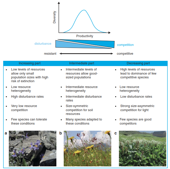
Fig. 20.18 Conceptual model to explain the hump-shaped productivity–diversity relationship. The table summarises the main postulated mechanisms leading to the hump-shaped curve. The photos show some examples that are typical for the three parts of the hump. a Linaria alpina, a pioneer species colonising a heavily disturbed rock fan with minor amounts of mineral soil in the Swiss Alps. b Highly diverse, extensively managed subalpine meadow in the Swiss Alps, with intermediate levels of soil resource availability (low fertiliser input) and disturbance (cutting, grazing). c Rumex alpinus (foreground) dominates a patch in an alpine pasture, with high inputs of nutrients from resting livestock (“Lägerflur”).

With increasing levels of resources and lowering levels of disturbance, more and more species are able to establish and to build up stable population sizes, and more biomass can be produced. Nutrient availability is still rather low at the increasing and plateau part of the hump, and plants mainly size-symmetrically compete for soil resources (i.e. species with larger root systems acquire more resources than those with smaller ones), which does not lead to competitive exclusion (Cahill 1999). At high levels of resource availability, coupled with low disturbance frequency and intensity, tall and highly competitive species produce closed canopies, diminishing light availability in the understorey. Competition for light is now more important than that for soil resources, and less competitive species are excluded, so diversity declines. This pre-emption of light is a good example of size- asymmetric competition for a resource of directional supply (Sect. 19.3).

This proposed mechanism explaining the decreasing part of the hump has been supported by a somehow simple, but clever, experiment. Hautier, Niklaus and Hector (2009) assembled grassland communities in a glasshouse, fertilised them and added light to the understorey (Fig. 20.19). As expected, fertilisation increased biomass production and canopy height and decreased light levels in the understorey. In consequence, this resulted in a loss of low-statured perennial grasses and herb species. Adding light to the understorey in the fertilised plots, however, reduced competition for light and maintained plant diversity. Thus, by combining fertilisation with light addition in a full factorial design, the researchers could show that competition for light did indeed result in a loss of plant species in the face of eutrophication and related increases in productivity. From an applied perspective, this experiment gives clear arguments to prevent or reduce eutrophication owing to a surplus of fertilisers or atmospheric deposition if biodiversity is to be protected or restored, especially in nutrient- limited, species-rich ecosystems (Fig. 20.18).

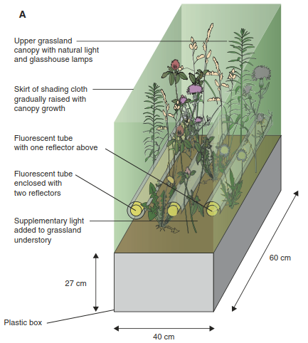
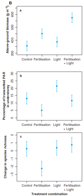
Fig. 20.19. Experimentally testing the decrease of species richness under high productivity levels. The experiment involved manipulation of soil nutrient levels and understorey light conditions in grassland model ecosystems. The four treatment combinations were “control” (unfertilised, closed lights), “fertilisation” (fertilised, closed lights), “light” (unfertilised, open lights) and “fertilisation + light” (fertilised, open lights). A Experimental set-up; for illustration purposes only, two open lights and one closed light are shown in the same experimental unit, but they were installed in different treatments. B Above-ground biomass production a, light availability in the understorey b, and change in plant species richness c in response to the experimental treatments. Points denote treatment means, and the intervals show least significant differences (treatments with non- overlapping intervals are significantly different at p = 0.05). PAR: photosyn-thetically active radiation (Hautier et al. 2009). Reproduced with permission from AAAS

Despite the fact that the humped-shaped relationship between productivity and diversity has been documented often, controversy remains about the generality of this pattern, its dependence on spatial scale, the history of community assembly, measures of productivity or other methodological inconsistencies. For example, two large-scale, global studies that applied standardised sampling designs found either general support for the humped-shaped relationship in grassland communities (Fraser et al. 2015) or no significant relationship between peak aboveground live biomass and fine-scale plant species richness (Adler et al. 2011). The differences between both studies might be due to different statistical approaches or to the inclusion/exclusion of highly productive sites, which were found to be very low in species richness, thus strongly influencing the decreasing part of the hump in the Fraser et al. (2015) study. But despite these differences, both studies showed that the humped-back model has quite low explanatory power, even if the relationship as such remains significant. Rather, it seems that productivity and richness are both influenced by a multitude of factors and processes, such as nutrient supply rates, disturbance, habitat heterogeneity, assembly history or management. Thus, instead of focusing too narrowly on bivariate patterns such as the hump-shaped curve, future investigations should look into multivariate mechanisms controlling plant diversity.