Box 20.1: Quantification of Biodiversity

How diverse is an ecosystem, and does this diversity change over time? Do distinct landscapes differ in their biodiversity? Which aspect of biodiversity responds first to changes in environmental conditions or management? To answer such typical questions in ecology, biodiversity must be quantified. However, the concept of biodiversity with its numerous facets is difficult to handle without proper definition and measures.

In essence, any measure of biodiversity should encompass the richness of different entities, and the degree of difference or dissimilarity between those entities, for example, species in a sample or in a community. One way to represent the differences between such entities is to account for the relative abundance or evenness of those entities. Other ways to differentiate between entities include aspects of genetics, morphology, biochemistry, biogeography or the functional role within ecosystems. Therefore, it has to be noted that “there is no single all-embracing measure of biodiversity—nor will there ever be one!” (Gaston and Spicer 2004).

The measure of species richness is simply the total number of species within a sample or community. The number of individuals of each species is irrelevant for this measure. If the number of species is related to an area (e.g. per square metre), the term species density is also used.

To distinguish diversity at different spatial scales, the concept introduced by Whittaker (1960) is often used, which distinguishes the following categories:
Point diversity: number of species in a small or micro-habitat sample, taken within a community regarded as homogeneous;
а-diversity: within-habitat diversity, that is, the number of species within a community and per area;
β-diversity: between-habitat diversity differentiation, that is, a dimensionless comparative number of species in different units of vegetation or habitats;

Y-diversity: landscape diversity, that is, the number of species in larger units, such as an island or landscapes that include more than one community.

Later, he added two levels at higher spatial scales, which, however, are rarely used:

δ-diversity: geographic diversity differentiation, that is, dimensionless comparative number of species applied to changes over large scales (e.g. along climatic gradients or between geographic areas); it is the functional equivalent of beta diversity at the higher organisational level of the landscape;

ε-diversity: regional diversity, that is, the total number of species in a broad geographic area, including different landscapes or groups of areas of gamma diversity.

a-, y- and ε-diversity are thus measured in particular areas, the first in those that are occupied by a community, the latter in larger spatial units, such as ecosystems, landscapes or regions. β- and δ-diversity, in contrast, must be calculated and describe changes in the number of species between habitats or landscapes or along ecological gradients. β-diversity may also be used for comparisons of number of species in the same habitat over time and is then a measure of species turnover.

Beside species richness, one of the most frequently used indices of diversity is that of Shannon and Weaver (1949):

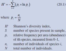
In this index, the richness and proportional abundance of species are included because both aspects determine the hetero- geneity—and therefore the diversity—of a community. H' rises with an increasing number of species or increasing uniformity of distribution of relative abundance (e.g. cover or biomass) of individual species. In habitats with single species, the value is zero. If all species have the same relative abundance, H' is at its maximum. Shannon’s index is independent of the functional characteristics of the individual species: all are treated equally.

The same index can also be used to calculate the genetic diversity within a population, with pi being the relative frequency of the ith allele.

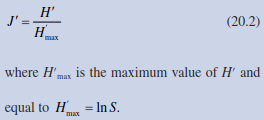
The Shannon indices of different communities do not tell us whether a high value is due to a higher number of species or to a more even distribution of individuals. To compare communities with different species richness, the evenness can be calculated, that is, the uniformity of species distribution in a habitat. Evenness indices reflect the ratio of dominant to rare species within a single value, and several such indices exist, all of which have specific features (Smith and Wilson 1996). The index by Pielou (1966) is based on Shannon’s index:

To describe the dominance distribution of species within a community, indices can be used that give more weight to the more abundant species, while the addition of rare species results in only minor changes. Such an index is Simpson’s index (Simpson 1949), which describes the probability that two individuals randomly selected from a sample will belong to the same species:

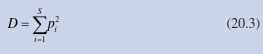
To obtain an increasing value with increasing diversity, this index is most often presented as Simpson’s index of diversity 1 - D (ranging from 0 to 1) or as Simpson’s reciprocal index 1/D.

To describe the similarity or dissimilarity in species composition between different flo- ristic regions, plant communities or sample quadrats, several indices have been developed, for example:

The Jaccard similarity coefficient, which uses information on species absence or presence in two samples (Jaccard 1912):

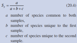
It is often multiplied by 100% and can also be presented as an index of dissimilarity by

Very similar is the S0rensen-Dice similarity coefficient, which gives more weight to species common in both samples (Dice 1945; S0rensen 1948):

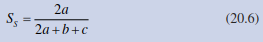
As with the Jaccard index, it can also be expressed as a percentage, or as dissimilarity, the latter representing the Bray-Curtis dissimilarity (Bray and Curtis 1957):

This index is bound between 1 and 0, with 1 representing a situation where the two samples do not share any species, and 0 meaning the two samples have identical species compositions.

Other indices to compare species compositions have been developed, for example, by including information on abundances, by generalising to more than two samples or by using other distance measures such as Euclidean distances. More details can be found in textbooks dealing with analyses of ecological data (e.g. Legendre and Legendre 2012).