Environmental Gradients and Plant Community Distributions

Theoretical Foundations: Organismal vs. Individualistic Paradigms. Much of the history of plant ecology has been dominated by a foundational debate regarding the fundamental nature of plant communities and the mechanisms by which plant populations group into distinct associations (McIntosh 1981, 1985; Golley 1993). Historically, two main polar paradigms emerged to explain these patterns:

- The Organismal Concept (Clementsian School): One school of thought held that communities are emergent units representing a distinct, higher level of ecological organization (Clements 1916, 1928; Odum 1953, 1969, 1971). In this classical organismal view, plant species are tightly integrated, co-evolved assemblages functioning analogously to a complex superorganism with discrete spatial boundaries.

- The Individualistic Concept (Gleasonian School): A second, opposing school viewed communities merely as temporally and spatially co-occurring species (Gleason 1917, 1926, 1939). Proponents maintained that plant communities are not emergent biological units, but rather consist simply of independent species that happen to exhibit similar environmental tolerances, physiological requirements, and habitat preferences.

Numerous empirical studies of vegetation distribution along environmental gradients, particularly within complex mountain ecosystems, have demonstrated the validity of the individualistic paradigm. Our modern understanding of plant community dynamics confirms that floristic composition changes continuously along environmental gradients rather than discretely. This continuous shift produces a continuum of populations rather than a sharp series of distinct plant associations. Plant species do not aggregate into fixed, closed ecological units; instead, they distribute individualistically according to their inherent ecophysiology, reproductive strategies, and life history patterns. Communities exhibiting recognizable floristic composition and physiognomy merely form from the overlapping geographic distributions of species. Consequently, vegetation classification units such as "communities" serve as convenient, arbitrary constructs of ecological taxonomy rather than discrete, self-bounding entities in nature.

Empirical Gradient Analysis in the Great Smoky Mountains. The continuum concept of vegetation is clearly demonstrated in the spatial dispersion of plant species along steep abiotic gradients. The vegetation of the Great Smoky Mountains along the Tennessee–North Carolina state border provides an exemplary model of plant distribution along environmental gradients (Whittaker 1956). Within this region, topographical elevation ranges from 460 m in the alluvial bottomlands to 2000 m at the summits of the highest peaks. This topographical relief drives strong microclimatic variations: annual precipitation increases from less than 1500 mm in the lower valleys to more than 2000 mm at high elevations.

The relative abundance of tree species changes markedly across this vertical gradient (Figure 19.7). When mapped against elevation, individual species distributions exhibit characteristic bell-shaped or rounded curves. These population curves overlap broadly with neighboring species, yet maintain distinct, species-specific modal centers along the gradient:

- Low-Elevation Mesic Sites: Dominated primarily by yellow poplar (Liriodendron tulipifera).
- Mid-Elevation Mesic Sites: Yellow birch (Betula allegheniensis), mountain silverbell (Halesia tetraptera), sugar maple (Acer saccharum), white basswood (Tilia americana), and yellow buckeye (Aesculus flava) become progressively dominant.
- High-Elevation Sites (>1400 m): Transitions almost exclusively into high-altitude American beech (Fagus grandifolia) forests.

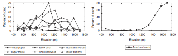
Figure 19.7. Distribution of tree species, as a percentage of the number of trees in the stand, in relation to elevation on mesic sites in the Great Smoky Mountains circa 1940s and 1950s. Data from Whittaker (1956).

On xeric (dry) topographic sites, the floristic composition differs substantially, consisting predominantly of oak and pine forest complexes (Figure 19.8). The dominant oak species include blackjack oak (Quercus marilandica), chestnut oak (Quercus montana), and scarlet oak (Quercus coccinea). Concurrently, Virginia pine (Pinus virginiana), pitch pine (Pinus rigida), and table mountain pine (Pinus pungens) are highly abundant:

- Low-Elevation Xeric Sites: Virginia pine and blackjack oak grow almost exclusively at elevations less than 800 m.
- Intermediate Elevations: Pitch pine and table mountain pine dominate in complex association with scarlet oak and chestnut oak.
- High-Elevation Xeric Ridges: Table mountain pine dominates the forest canopy alongside minor proportions of chestnut oak and pitch pine.

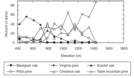
Figure 19.8. As in Figure 19.7, but for xeric sites.

Community Classification, Structural Physiognomy, and Topography. Despite the continuous nature of plant distributions, vegetation can be categorized into distinct community types or associations for analytical purposes based on physiognomy and floristic composition.

- Physiognomy: Refers to the physical structure, architecture, and growth form of the vegetation (e.g., woody vs. herbaceous layers, canopy overstory, understory stratification).
- Floristic Composition: Focuses on the specific taxonomic identity and relative abundance of dominant canopy species (e.g., oak-hickory vs. spruce-fir associations).

In the Great Smoky Mountains, multiple plant communities segregate systematically across topographic moisture and elevation gradients (Figure 19.9):

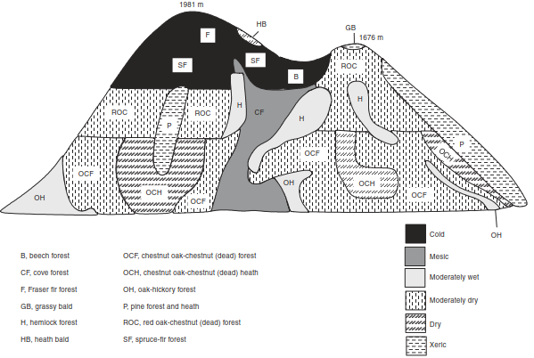
Figure 19.9. Topographic distribution of vegetation types on a west-facing slope in the Great Smoky Mountains circa 1940s and 1950s. Adapted from Whittaker (1956).

At high-altitude extremes, unique specialized habitats emerge: exposure-resistant heath balds dominated by evergreen ericaceous shrubs occupy dry, wind-exposed ridges, whereas high-altitude summits feature expansive grassy balds.

Dominance-Diversity Dynamics and Environmental Niches. Although one or two canopy-dominant species often define the visual physiognomy of a forest, most plant communities in the Great Smoky Mountains comprise multi-species assemblages. This community structure is formally evaluated using dominance-diversity curves, which plot the relative importance (percentage of total trees in a stand) of each species ranked from most to least abundant (Figure 19.10).

In sheltered south-facing slopes above 1372 m, American beech exhibits extreme dominance, accounting for 81% of all trees with a diameter at breast height (DBH) greater than 2.54 cm. Secondary species in these high-altitude beech forests include mountain silverbell (8%), followed by yellow birch and yellow buckeye (combining for 5%).

Conversely, mid-elevation cove forests between 762 m and 1067 m display significantly higher species evenness and functional diversity. Four co-dominant species—mountain silverbell, white basswood, sugar maple, and yellow birch—collectively account for 69% of the canopy trees, while six additional tree species (each contributing 2–6% relative abundance) account for the remaining 21% of the forest stand.

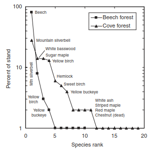
Figure 19.10. Dominance–diversity curves for beech forests growing on sheltered south slopes above 1372 m and cove forests between 762 and 1067 m in the Great Smoky Mountains circa 1940s and 1950s. Graphs show the relative importance of species, in terms of percentage of trees in the stand, ranked from most important to least important. Data from Whittaker (1956).

Species Realized Niches along Bivariate Gradients. Two-dimensional ecological contour mapping confirms that most tree species exist along a spatial and environmental continuum (Figure 19.11). While certain species exhibit narrow ecological amplitude—such as white basswood, which is strictly confined to sheltered, moist cove forests—most major tree species span multiple plant associations:

- Chestnut Oak (Quercus montana): Achieves its highest population density in chestnut oak communities, yet maintains populations exceeding 5% abundance across adjacent oak-hickory and xeric pine forests.

- Eastern Hemlock (Tsuga canadensis): Reaches maximum density in cool hemlock ravines, but maintains abundances greater than 10% in surrounding cove forests and moist oak-hickory stands.

- Red Maple (Acer rubrum): Acts as a generalist species that rarely forms a single, distinct community type; instead, it intermingles across almost all elevation and moisture regimes.

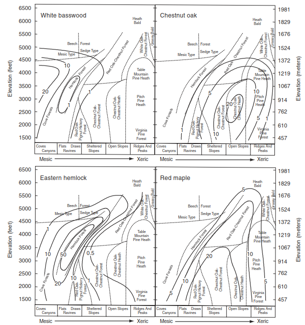
Figure 19.11. Population distributions for white basswood, chestnut oak, eastern hemlock, and red maple in relation to elevation and moisture in the Great Smoky Mountains circa 1940s and 1950s. Contour lines show species abundance in terms of percentage of trees. Major vegetation types are delimited. Adapted from Whittaker (1956).

Ultimately, these empirical observations validate the individualistic hypothesis: plant species respond independently to complex environmental gradients of moisture, temperature, and elevation according to their specific physiological thresholds, resulting in overlapping, continuous vegetational patterns across the landscape.