Canopy Turbulence Dynamics: Counter-Gradient Transport and Scalar Flux Modeling in Plant Canopies

Many standard models of turbulent fluxes in plant canopies utilize the principle of diffusion along the mean concentration gradient, similar to turbulent transport mechanisms in the atmospheric surface layer. In traditional micro-meteorology, the vertical fluxes of momentum, sensible heat, and water vapor are assumed to be directly proportional to the vertical gradients of mean horizontal wind speed, potential temperature, and specific humidity, respectively, multiplied by a turbulent diffusivity (also referred to as aerodynamic conductance).

However, Monin–Obukhov stability theory breaks down in the layer of air located immediately above and within the vegetative canopy, designated as the roughness sublayer. In this regime, universal similarity functions lose their validity. The classic gradient-diffusion approach (commonly known as K-theory) fails within plant canopies due to the widespread occurrence of counter-gradient transport, zero-gradient fluxes, and highly intermittent turbulence (Denmead and Bradley 1985; Raupach and Finnigan 1988; Baldocchi 1989; Baldocchi and Meyers 1998; Finnigan 2000).

To overcome the inherent limitations of first-order gradient-diffusion formulations, advanced fluid dynamics models are required to represent canopy micro-meteorology accurately. These modeling paradigms include higher-order closure models—which evaluate first-order moments (such as mean horizontal wind velocity and mean scalar mixing ratio) along with second-order moments (such as vertical velocity variance and covariances of mixing ratio and vertical velocity fluctuations)—and Lagrangian stochastic models that track individual particle trajectories within canopy flow fields (Wilson and Shaw 1977; Meyers and Paw U 1986, 1987; Wilson 1988; Baldocchi 1992; Pyles et al. 2000).

Micro-Meteorological Turbulence in Deciduous Forest Canopies. Empirical studies conducted in a temperate deciduous forest provide clear illustrations of the complex hydrodynamic challenges involved in modeling turbulent transfer (Baldocchi and Meyers 1988a,b, 1989; Meyers and Baldocchi 1991). The studied stand consisted primarily of oak (Quercus) and hickory (Carya) species, featuring a total canopy height of h ≈ 23 m and an overall leaf area index (LAI) of approximately 5 m² m⁻².

Spatial leaf area distribution was heavily skewed toward the upper canopy: over 75 percent of the total leaf area resided within the upper 25 percent of the canopy height (the top 5 m). Detailed micro-meteorological measurements within this structural profile revealed an extraordinarily complex turbulent flow structure characterized by high temporal intermittency, large coherent eddies, and non-Gaussian velocity probability density functions.

Wind speed within the canopy varies with height in direct relation to the profile of leaf area index (Fig. 17.11).

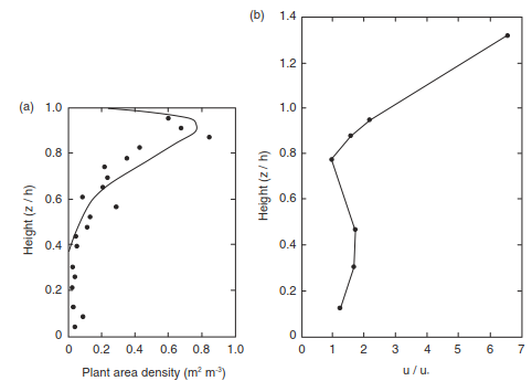
Fig. 17.11. Profiles of (a) leaf area and (b) wind speed above and in the canopy of a deciduous forest. Height (z) is given as a fraction of canopy height (h). Wind speed is normalized by friction velocity (u) measured above the canopy. Adapted from Baldocchi and Meyers (1988a) and Baldocchi (1989).*

As illustrated in Fig. 17.11, intense wind shear occurs near the canopy top above 0.8h, where leaf foliage is densest. Within this region, mean horizontal wind speed decreases rapidly with depth due to aerodynamic drag exerted by foliage. Below this height, an inflection in the vertical wind velocity profile occurs, giving rise to a localized velocity maximum around 0.5h, followed by a secondary decline toward the forest floor. This non-monotonic profile contradicts simple exponential wind decay assumptions and clearly demonstrates counter-gradient momentum transport.

Scalar Fluxes and Counter-Gradient Transport Dynamics. Comprehensive field studies by Denmead and Bradley (1985) in a ponderosa pine (Pinus ponderosa) forest provided direct empirical evidence of counter-gradient and zero-gradient scalar fluxes. Profiles of potential temperature, water vapor mixing ratio, and CO₂ concentration measured in the canopy are illustrated in Fig. 17.12.

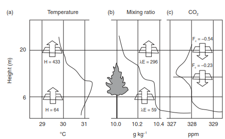
Fig. 17.12. Mean profiles of (a) potential temperature, (b) water vapor mixing ratio, and (c) CO₂ concentration observed in a ponderosa pine forest over a period of one hour. Also shown are the fluxes of sensible heat (H, W m⁻²), latent heat (λE, W m⁻²), and CO₂ (F꜀, mg m⁻² s⁻¹) at two heights in the canopy. Adapted from Denmead and Bradley (1985).

As detailed in Fig. 17.12, mean potential temperature exhibits a maximum near the middle of the canopy. The water vapor mixing ratio decreases from a high near the surface, is nearly constant with height in the lower canopy space, and decreases with height in the upper canopy. The concentration of CO₂ has a minimum in the middle of the canopy due to intense photosynthetic assimilation by active foliage.

Standard gradient-diffusion theory predicts that sensible heat should flow upward above the mid-canopy temperature maximum and downward onto the forest floor below mid-canopy. Likewise, the steep gradient of water vapor near the forest floor suggests enhanced evaporation from the forest floor, while the CO₂ profile implies upward transport of CO₂ from the forest floor in the lower canopy and downward flux of CO₂ in the upper canopy.

However, observed turbulent flux measurements depart markedly from conventional expectations:
- Upper Canopy Dynamics: Observed fluxes in the upper canopy conform to conventional gradient-diffusion relationships. Upward fluxes of sensible heat (H = 433 W m⁻²) and water vapor (λE = 296 W m⁻²) are accompanied by negative gradients of temperature and water vapor. The downward flux of CO₂ (F_с = -0.54 mg m⁻² s⁻¹) occurs along a positive concentration gradient.

- Lower Canopy Anomalies: In the lower canopy, however, these fluxes are associated with counter-gradients or zero-gradients. Downward flux of CO₂ (F_с = -0.23 mg m⁻² s⁻¹) occurs along a positive concentration gradient. Sensible heat flux is upward (H = 64 W m⁻²) even though temperature increases with height. Furthermore, a large upward flux of water vapor (λE = 59 W m⁻²) occurs despite zero gradient. Substantial absorption of CO₂ occurs below the middle of the canopy.

These counter-gradient transport phenomena are driven by large-scale, intermittent turbulent eddies originating above the canopy height (h). These coherent structures penetrate deep into the trunk space, sweeping scalar quantities across large vertical distances independent of local gradient conditions.

Resistor Network Models of Canopy Mass and Energy Exchange. To parameterize scalar fluxes across soil-vegetation-atmosphere continua without relying on invalid gradient-diffusion assumptions, multi-layer and multi-source conductance networks are widely implemented, as depicted in Fig. 17.13.

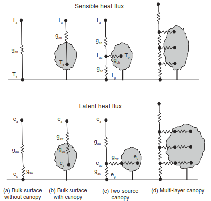
Fig. 17.13. Conductance networks for sensible heat flux (top) and latent heat flux (bottom). Networks are for a bulk surface without a canopy, vegetation with a bulk surface formulation, a two-source canopy, and multiple canopy layers. (a) The surface is the ground and fluxes are regulated by aerodynamic conductances (gₐₕ, gₐ{w}). Latent heat flux also includes a soil conductance (g_g). (b) The bulk canopy uses an effective surface temperature (Tₛ) and vapor pressure (eₛ) that combines vegetation and ground. The overall conductance for latent heat is a surface conductance (gₛ{w}) acting in series with an aerodynamic conductance (gₐ{w}). (c) The two-source canopy partitions fluxes into vegetation and ground based on vegetation (Tᵥ, eᵥ) and ground (T_g, e_g) temperature and vapor pressure. The conductance gₐ_с accounts for aerodynamic processes within the canopy. Canopy conductances account for sensible heat exchange (g_ch) from the vegetation to air within the canopy (Tₐ_с) and latent heat exchange (g_cw) from the vegetation to canopy air (eₐ_с). For latent heat, this also includes stomatal conductance. (d) Multiple canopy layers.

As illustrated in Fig. 17.13, resistance schemes range in complexity depending on vertical structure:
1. Bulk Surface Without Canopy: The surface is the ground, and sensible/latent heat fluxes are regulated directly by aerodynamic conductances (gₐₕ, gₐ{w}). Latent heat flux also incorporates soil surface conductance (g_g).

2. Bulk Surface With Canopy: Uses an effective surface temperature (Tₛ) and vapor pressure (eₛ) combining vegetation and ground. The overall conductance for latent heat is a surface conductance (g⛛{w}) acting in series with an atmospheric aerodynamic conductance (gₐ{w}).

3. Two-Source Canopy Models: Partition fluxes into vegetation and ground components based on vegetation (Tᵥ, eᵥ) and ground (T_g, e_g) temperature and vapor pressure. The conductance gₐ_с accounts for aerodynamic transport processes within the canopy space. Canopy conductances account for sensible heat exchange (g_ch) from vegetation to canopy air (Tₐ_с) and latent heat exchange (g_cw) from vegetation to canopy air (eₐ_с), which includes stomatal conductance.

4. Multi-Layer Canopy Frameworks: Discretize the vertical canopy architecture into multiple computational layers (i = 1, 2, …, n). Each layer independently resolves leaf energy balances, micro-environmental scalar profiles, radiation absorption, and stomatal conductance responses.

By integrating multi-layer conductance networks with higher-order closure schemes or Lagrangian stochastic frameworks, modern atmospheric transport models can accurately resolve the complex coupling of canopy turbulence, stomatal physiology, and surface-atmosphere energy exchange.