Modeling Canopy Energy Fluxes and Aerodynamic Conductance

Introduction to Vegetation-Atmosphere Energy Exchange. The fundamental biophysical principles that govern temperature regulation and energy fluxes at the individual leaf scale also dictate energy dynamics across entire vegetated surfaces. Modeling turbulent fluxes between land surfaces and the atmospheric boundary layer requires precise formulations of thermal and hydrological transfer processes. Figure 17.13 illustrates several standard approaches used to model these turbulent exchanges within land-surface parameterization schemes.

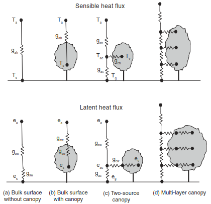
Fig. 17.13. Schematic representations of turbulent flux modeling across vegetated surfaces.

A foundational approach relies on a bulk aerodynamic formulation, which parameterizes turbulent transfer using a single aerodynamic conductance operating between the surface and the atmosphere. To account for unsaturated soil conditions, a distinct soil conductance is introduced to regulate moisture transport from ground level.

Big-Leaf Canopy Formulations and Radiometric Temperature. Principles of the Big-Leaf Model. The influence of vegetation on surface fluxes can be included by treating the soil–canopy system as an effective bulk surface (Figure 17.13b). This formulation, known as the big-leaf model, conceptualizes the entire plant canopy as a single scaled leaf. In this scheme, radiative exchange is integrated over the total canopy, and leaf-level conductances are aggregated to represent whole-canopy conductance.

Mathematical equations governing canopy energy fluxes in a big-leaf model parallel individual leaf energy balance equations. Latent heat flux is routinely calculated using the Penman-Monteith equation, which acts as a classic big-leaf representation by scaling stomatal and boundary layer conductances across the canopy layer.

Surface and Radiometric Temperature Parameters. Bulk surface models are extensively deployed to monitor plant canopies. When sensible heat flux (H) and aerodynamic conductance are derived from micrometeorological measurements, the effective aerodynamic surface temperature (Ts​) can be estimated via the bulk aerodynamic formula for sensible heat:

In Equation (17.19), Tₐ represents ambient air temperature, cₚ denotes the volumetric specific heat capacity of air, and gₐₕ is the aerodynamic conductance for heat. Alternatively, Tₛ can be inferred from measurements of upward longwave radiation, yielding the radiometric temperature, which corresponds to the equivalent surface temperature emitting thermal longwave radiation.

Roughness Lengths and Excess Resistance. Discrepancy Between Momentum and Heat Transfer. Applying bulk aerodynamic formulas requires distinguishing between the roughness length for momentum (z₀ₘ) and the roughness length for heat (z₀ₕ). Because momentum transfer occurs via pressure forces across obstacles while heat transfer depends strictly on molecular diffusion across thin boundary layers, z₀ₕ is typically smaller than z₀ₘ (Thom 1972; Garratt and Hicks 1973; Garratt 1978; Beljaars and Holtslag 1991).

Failing to account for this difference introduces substantial errors in surface temperature estimates derived from sensible heat flux. Consider a forest canopy with height h = 20 m, displacement height d = 14 m, z₀ₘ = 2 m, and z₀ₕ = 0.2 m. Under a wind speed u = 2 m s⁻¹ at height z = 30 m (neglecting atmospheric stability effects), the aerodynamic conductances calculated for momentum (gₐₘ) and heat (gₐₕ) yield gₐₘ = 3.1 mol m⁻² s⁻¹ and gₐₕ = 1.5 mol m⁻² s⁻¹.

Quantifying Excess Resistance. The reduction in heat conductance relative to momentum transfer represents an excess resistance (1 / gᵦ* = 1 / gₐₕ - 1 / gₐₘ = 2.8 mol⁻¹ m² s), expressed generally as:

Where ρₘ is the molar density of air, k is the von Kármán constant, and u* is the friction velocity (u* = 0.385 m s⁻¹). This excess resistance creates a temperature difference between height z₀ₕ and z₀ₘ. For example, assuming H = 200 W m⁻² and Tₐ = 30°C, the temperature at z₀ₕ evaluated via Equation (17.19) is Tₛ = 34.6°C (with cₚ = 29.2 J mol⁻¹ K⁻¹), whereas Tₛ evaluated at z₀ₘ using gₐₘ is 32.2°C. The temperature difference between these reference heights is modeled by:

Here, θ* = -H / (ρₘ cₚ u*), yielding θ* = -0.42 K with ρₘ = 42.3 mol m⁻³.

Vegetation Canopy Architecture and Thermal Coupling. Tall Forests vs. Short Vegetation Dynamics. By influencing aerodynamic conductance, the height of plants has a large influence on leaf temperature. Tall forest vegetation is aerodynamically rough and features elevated aerodynamic conductance. Consequently, heat is readily exchanged with the atmosphere, and the temperature of leaves is closely coupled to that of the air.

In contrast, short vegetation such as grass or shrub is aerodynamically smooth, displays low aerodynamic conductance, and dissipates heat less effectively. The leaves of short vegetation are decoupled from the air and have warmer temperatures than that of the air. In cold climates, short stature may convey an advantage by warming leaf temperature (Wilson et al. 1987; Grace 1988; Grace et al. 1989).

Figure 17.14 illustrates this for alpine forest and shrub vegetation across net radiation gradients. For both types of vegetation, the leaf-to-air temperature difference increases with greater net radiation. In the tall forest, the slope of this relationship is small, keeping leaf temperatures similar to air temperature with a maximum excess of less than 5°C. In the dwarf shrub vegetation, the slope is larger and the temperature excess is 15°C in bright sunshine.

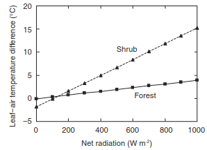
Fig. 17.14. Relationship between daytime leaf–air temperature difference and net radiation for forest (15–18 m tall) and dwarf shrub (0.1 m tall) vegetation. Data are shown for wind speeds of 1–3 m s⁻¹. Data from Grace et al. (1989).

Multi-Source Canopy Models and Energy Balance Solvers. Two-Source Energy Partitioning. As an alternative to the bulk representation of the effective surface for heat and moisture exchange, the surface can be explicitly represented by ground and vegetation (Figure 17.13c). Sensible heat flux is partitioned into that from foliage (Hᵥ), that from ground (H_g), and that from canopy air to the atmosphere (H), each regulated by different processes. The leaf boundary layer conductance (g_ch) scaled to the canopy governs sensible heat flux from foliage, while turbulent processes within the canopy govern sensible heat flux from the soil (H_g).

Latent heat is partitioned into soil evaporation and transpiration. Transpiration is regulated by a canopy conductance that is an integration of leaf boundary layer and stomatal conductances over all the leaves in the canopy. Soil evaporation is regulated by aerodynamic processes within the plant canopy and by soil moisture. These equations can be solved by writing the sensible and latent heat fluxes as a linear combination of atmospheric, vegetation, and ground temperatures and vapor pressure, respectively (Deardorff 1978).

Assuming the canopy air has negligible capacity to store heat, the total sensible heat flux to the atmosphere is the sum of fluxes from vegetation and the ground:

Rearranging terms in these equations, the canopy air temperature (Tₐ_c), which is common to all three fluxes, is evaluated as a weighted average of the atmospheric (Tₐ), vegetation (Tᵥ), and ground temperatures (T_g):

This equation for canopy air temperature is substituted into the expression for latent heat flux from vegetation (Hᵥ). A similar equation is derived for canopy air vapor pressure (eₐ_c) for latent heat flux, and the energy balance of the canopy is solved for the temperature (Tᵥ) that balances net radiation, sensible heat flux, and latent heat flux. Then, with canopy fluxes known, the ground fluxes and temperature (T_g) are updated.

Canopy Thermal Storage and Microclimate Profiles. Alternatively, one can assume that the canopy air has some capacity to store heat (Vidale and Stöckli 2005). The storage of heat in the canopy air is:

where ∂T / ∂t is the rate of change of temperature (K s⁻¹) and ∂z is canopy height (m). For a canopy with a height z = 25 m, a change in temperature of 1°C hr⁻¹ is associated with approximately 8 W m⁻² heat storage in the canopy. If heat storage is included, the canopy air temperature is not diagnosed as a linear combination of Tₐ, Tᵥ, and T_g as above, but rather predicted from:

The storage heat in the canopy air space is the difference between heat entering the air space (Hᵥ, H_g) and sensible heat transferred to the atmosphere (H).

Figure 17.15 illustrates the average diurnal cycle of CO₂ concentration within and above a 70-year-old quaking aspen forest with a canopy height of 21.5 m when leafless and in full leaf (Yang et al. 1999). During full-leaf conditions, daytime uptake reduces CO₂ concentrations inside the canopy, while nighttime respiration leads to significant accumulation of CO₂ near the ground level (0.8 m).

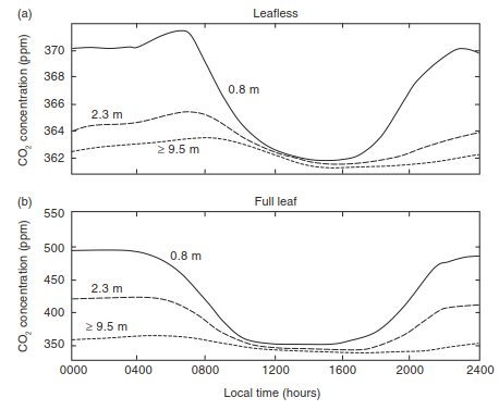
Fig. 17.15. Average diurnal cycle of CO₂ concentration within and above a 70-year-old quaking aspen forest with a canopy height of 21.5 m when (a) leafless and (b) in full leaf. Adapted from Yang et al. (1999).

The preceding methodologies provide simple means to simulate fluxes from plant canopies and are commonly used in climate models (Deardorff 1978; Dickinson et al. 1986, 1993; Sellers et al. 1986, 1996a,b). They can be extended to represent multiple canopy layers (Figure 17.13d) with a simple representation of aerodynamic conductances within the canopy (Shuttleworth and Wallace 1985; Choudhury and Monteith 1988). However, two-source canopy models and multilayer models are based on gradient-diffusion theory and do not allow for counter-gradient fluxes as observed in plant canopies. More complex canopy models are required to resolve turbulent fluxes in plant canopies (Baldocchi 1992; Baldocchi and Meyers 1998; Pyles et al. 2000).