Satellite Data Integration in Global Land Surface Modeling

Integration of Satellite Remote Sensing Data in Land Models. The evolution of land surface models has historically proceeded in direct tandem with the availability of global land data products derived from Earth-observing satellites. Early generation land surface models relied on static, pre-existing geographic atlases and maps to prescribe spatial vegetation distributions (Matthews 1983; Olson et al. 1983; Wilson and Henderson-Sellers 1985; Dorman and Sellers 1989). Modern modeling frameworks dynamically integrate remotely sensed satellite observations to characterize key ecological surface variables, including land cover classification, leaf area index (LAI), and fractional vegetation cover (FVC).

Evolution of Satellite Land Cover Datasets. Global observations derived from spaceborne sensors became widely accessible for land modeling beginning in the mid-1990s. Numerical models require explicit surface characterization to define underlying biome distributions and biophysical surface parameterizations.

· Coarse Spatial Resolutions: Initial global datasets were constructed at a 1° spatial resolution (DeFries and Townshend 1994).

· High-Resolution Advancements: Subsequent remote sensing products provided improved grid scales at 8-km resolution (DeFries et al. 1998) and 1-km resolution (Loveland et al. 2000; Hansen et al. 2000; Friedl et al. 2002).

· Optical Biophysical Indicators: Datasets quantifying leaf area index (LAI) and the fraction of absorbed photosynthetically active radiation (FPAR) were developed at global grids of 1° (Sellers et al. 1994, 1996b), 0.5° (Nemani et al. 1996), and 8-km (Myneni et al. 1997; Buermann et al. 2002).

The second iteration of the Simple Biosphere Model (SiB2) was specifically re-engineered to ingest these continuous satellite observations (Sellers et al. 1996c). Implementing spaceborne vegetation products directly into coupled general circulation models yielded substantial improvements in simulated regional climate dynamics (Chase et al. 1996; Randall et al. 1996; Bounoua et al. 2000; Buermann et al. 2001).

Fractional Vegetation Cover and Canopy Heterogeneity. Surface models partition grid cell area using fractional vegetation cover to distinguish energy and moisture fluxes originating from transpiring vegetation versus bare soil substrate. Deardorff (1978) established the foundational formulation for fractional canopy coverage, which was later adopted by second-generation schemes such as BATS and SiB. These parameterizations initially prescribed fixed seasonal coverage values categorized strictly by biome type (Dickinson et al. 1986, 1993; Dorman and Sellers 1989).

Continuous global satellite measurements of fractional vegetation cover were subsequently generated at spatial scales of 1-km (DeFries et al. 1999; Zeng et al. 2000), 8-km (Zeng et al. 2003), and 0.15° (Gutman and Ignatov 1998). Integrating explicit continuous cover maps significantly enhanced the accuracy of terrestrial hydrological and thermal surface boundary simulations (Barlage and Zeng 2004).

Modeling Challenges in Sparse and Partial Vegetation Cover. Parameterizing sparse or partial canopy cover introduces significant structural complexity into physical numerical schemes. Early frameworks like BATS and SiB accommodated seasonal fluctuations in vegetated fraction and LAI, though the physical distinction between these two metrics remained poorly differentiated.

· Scale Dependencies: Forested landscapes exhibit structural gaps across localized scales (100–1000 m²) as well as extensive regional disturbances (10–100 km²) resulting from wildfires or harvesting.

· Homogeneous Big-Leaf Assumptions: Small-scale canopy openings are adequately captured using a big-leaf model representing a uniform forest stand, setting the fractional vegetation cover to 1 and setting the grid cell LAI equal to the local canopy LAI.

· Sub-Grid Patch Heterogeneity: Large open disturbances require explicit spatial partitioning into two discrete patches within a single grid cell: a dense vegetated patch and a bare soil patch. In this spatial formulation, the local LAI of the vegetated fraction exceeds the grid-cell average LAI.

· Arid Ecosystem Representations: Widely spaced vegetation in shrublands and desert scrub systems is accurately modeled as distinct, isolated vegetated patches separated by bare ground. Standard satellite FVC products primarily measure canopy sparseness rather than distinguishing between these structural canopy archetypes (Price 1992).

Integration of Photosynthetic Physiology and Carbon Dynamics. Earth system models have expanded beyond traditional hydrometeorological mechanics to incorporate stomata physiology, canopy photosynthesis, and the global terrestrial carbon cycle.

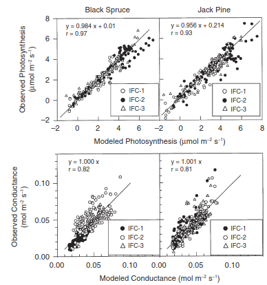
Fig. 25.4. Comparison between modeled and measured photosynthesis (top) and stomatal conductance (bottom) for branch samples of black spruce and jack pine trees. Data were collected during three intensive field campaigns (IFCs). Model parameters were derived for each IFC. Adapted from Dang et al. (1998).

Mechanistic parameterization of leaf-level physiology becomes complex in mixed life-form biomes, where co-occurring plant species exhibit fundamentally different photosynthetic rates, phenology schedules, carbon allocation strategies, and physiological traits. Aggregating morphologically distinct plant types into monolithic biomes creates mathematical inconsistencies with the underlying physiological equations.

Vegetation Continuous Fields and Plant Functional Types. To overcome the limitations of discrete land cover classes, vegetation continuous fields (VCF) were introduced to describe landscapes as continuous spatial gradients of plant functional traits (DeFries et al. 1995, 1997, 1999, 2000a,b; Hansen and DeFries 2004).

· Sub-Pixel Trait Mapping: Continuous field products map the fractional coverage of primary life forms within each pixel, such as tree canopy cover characterized at 1-km resolution by leaf longevity (evergreen vs. deciduous) and morphology (needleleaf vs. broadleaf).

· Multi-Class Ground Cover: Advanced 500-m resolution products differentiate tree canopy cover, bare ground, and non-tree herbaceous vegetation (Hansen et al. 2002, 2003).

· Plant Functional Types (PFTs): Continuous field data facilitate the subdivision of model grid cells into distinct Plant Functional Types. Standard numerical schemes establish seven primary PFT categories: needleleaf evergreen trees, needleleaf deciduous trees, broadleaf evergreen trees, broadleaf deciduous trees, shrubs, grasses, and crops (Bonan et al. 2002). Geographic variants (e.g., Arctic, boreal, temperate, and tropical biomes; C₃ and C₄ photosynthetic pathways) are categorized using biogeographical rules.

Disaggregating satellite-derived subpixel mosaics into distinct PFTs and leaf area indices remains computationally and algorithmically complex (Lawrence and Chase 2007). Because discrete PFTs simplify continuous trait variations across natural ecosystems, advanced modeling techniques incorporate continuous plant trait distributions to better capture ecological adaptation (Wang et al. 2012; Verheijen et al. 2013; Reich et al. 2014).