Modeling Terrestrial Ecosystems and Global Vegetation Dynamics

Biogeochemical and Dynamic Vegetation Models in Ecosystem Science. Terrestrial ecosystem modeling plays a pivotal role in understanding planetary ecology and biogeochemical cycling. Numerous numerical models have been developed to simulate net primary production (NPP), biomass accumulation, litterfall, and soil carbon in global terrestrial ecosystems. These models span a spectrum of scientific approaches, ranging from simple empirically based models to mechanistic process models of plant physiology and biogeochemical cycles. For example, empirical relationships (as shown in Fig. 24.4) have historically been used to model vegetation productivity in relation to temperature and precipitation (Esser 1987; Friedlingstein et al. 1992; Dai and Fung 1993; Post et al. 1997).

· Geographic Extent of Vegetation in Eastern North America

· Paleoclimate Reconstructions and Pollen Indicators

· Migration Patterns of Arboreal Species

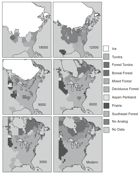
Fig. 24.17. Geographic extent of vegetation in eastern North America over the past 18 kyr BP. Vegetation types are based on pollen abundance. No analog means the pollen does not correspond to a modern vegetation type. Adapted from Overpeck et al. (1992) with graphics provided by the National Geophysical Data Center (National Oceanic and Atmospheric Administration, Boulder, Colorado).

Process models, however, are far more widely used than empirical models. Global models of terrestrial ecosystems generally fall into two broad classes: biogeochemical models and vegetation dynamics models.

Biogeochemical Ecosystem Models and Carbon Balance. Biogeochemical models simulate the carbon balance of ecosystems given a geographic distribution of vegetation, typically specified by biomes, as input to the model. These models employ specialized algorithms for photosynthesis, respiration, carbon allocation, and other plant physiological and microbial processes specific to different biomes. In these frameworks, vegetation is represented as aggregate pools of foliage, stem, and root biomass without regard to individual plants (as shown in Fig. 20.2).

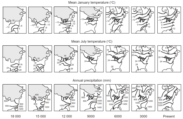
Fig. 24.18. Climate of eastern North America over the past 18 kyr BP reconstructed from pollen. The lightly shaded region shows the glacier. Adapted from Webb et al. (1993).

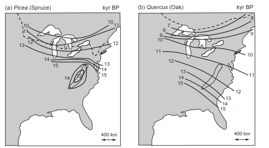
Fig. 24.19. Migration maps for (a) spruce and (b) oak. Contour lines show the time (kyr BP) of the first appearance of spruce or oak pollen in sediments. The dashed line shows the present southern range limit of spruce and northern range limit of oak. Adapted from Davis (1981).

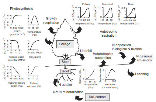
Fig. 24.20. Processes typically included in ecosystem models. Shown are the ecosystem carbon balance, environmental controls of photosynthesis and respiration, and internal carbon and nitrogen cycling.

One notable biogeochemical model is the Carnegie-Ames-Stanford Approach (CASA) model (Potter et al. 1993; Randerson et al. 1996). In the CASA model, net primary production is directly related to light-use efficiency, which is adjusted for temperature and soil moisture stress, solar radiation, and the fraction of photosynthetically active radiation absorbed by the canopy using Eq. (17.7). This absorption term is derived from satellite measurements of vegetation greenness, such as the normalized difference vegetation index (NDVI). Within the model framework, plant biomass is updated for NPP and associated litterfall, while soil carbon pools, nutrient mineralization, and nutrient allocation are calculated. The overall water balance is also simulated due to its fundamental control over net primary production and other ecological processes.

Another class of biogeochemical models explicitly links carbon fluxes with the water balance and nutrient cycling using mechanistic representations of net primary production and its environmental drivers. Examples of such global-scale ecosystem models include:

· The CENTURY model (Parton et al. 1987, 1988, 1993)

· The BIOME-BGC model (Running and Coughlan 1988; Running and Gower 1991; Running and Hunt 1993; Thornton et al. 2002)

· The Terrestrial Ecosystem Model (TEM) (Raich et al. 1991; McGuire et al. 1992; Melillo et al. 1993)

· The CASACNP model (Wang et al. 2010)

Physiologically based ecosystem process models simulate net primary production, decomposition, and nutrient availability in relation to leaf area index (LAI), biome type, and specific site conditions. These models incorporate light, temperature, water, and nutrient limitations to calculate net primary production, allocate carbon to grow foliage, stems, and roots, decompose litter, and mineralize nutrients (as shown in Fig. 24.20). Additionally, these models simulate leaf phenology based on prevailing environmental conditions. Typical phenological strategies include:

· Evergreen phenology, in which plants maintain foliage throughout the year

· Summergreen phenology, in which leaves are present during the warm season

· Raingreen phenology, in which foliage emerges during the rainy season and drops in the dry season

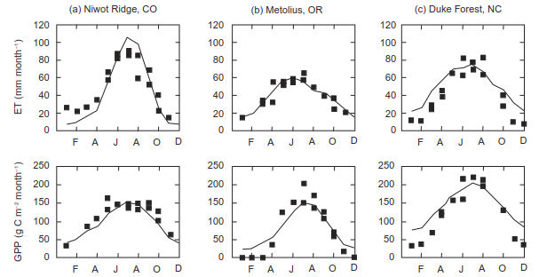
Fig. 24.21. Simulated (solid line) and observed (square) monthly evapotranspiration (top) and gross primary production (bottom) for three needleleaf evergreen forest sites in the United States. Adapted from Thornton et al. (2002).

Ecosystem models are routinely evaluated for their ability to simulate observed water and carbon fluxes. For example, Thornton et al. (2002) compared the BIOME-BGC model with eddy covariance measurements of evapotranspiration (ET) and carbon flux at several needleleaf evergreen forest sites across the United States. These validation sites included:

· Niwot Ridge, a 95-year-old subalpine conifer forest in Colorado (annual mean temperature: 2.1 °C, annual precipitation: 808 mm)

· Metolius, a mixed-age old ponderosa pine forest in Oregon (8.2 °C, 1251 mm)

· Duke Forest, a 17-year-old loblolly pine forest in North Carolina (14.6 °C, 1260 mm)

Across this broad climatic and stand-age gradient, the model reasonably captured monthly dynamics of evapotranspiration and gross primary production (GPP), despite minor discrepancies in specific months (as shown in Fig. 24.21).

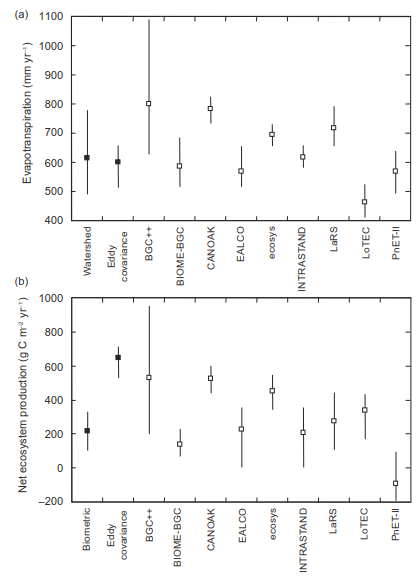
Fig. 24.22. Simulated and observed (a) annual evapotranspiration and (b) annual net ecosystem production for a broadleaf deciduous forest in the Walker Branch watershed near Oak Ridge, Tennessee. Data points are the mean (square) for the period 1993–2000. Also shown are the minimum and maximum annual fluxes (solid line). Observations are shown for two separate estimates. Model results are for nine ecosystem models. Data from Hanson et al. (2004).

In a comprehensive model comparison, Hanson et al. (2004) evaluated several ecosystem models against field observations at the Walker Branch watershed in Tennessee for the period 1993–2000. Watershed budget calculations of precipitation and runoff yielded a mean annual evapotranspiration of 613 mm yr⁻¹, while eddy covariance measurements indicated a similar mean of 601 mm yr⁻¹. Across nine distinct models, simulated mean annual evapotranspiration ranged from 463 to 801 mm yr⁻¹ (as shown in Fig. 24.22a). For carbon storage, mean annual net carbon storage derived from two biometric analyses was 218 g C m⁻² yr⁻¹, whereas mean carbon uptake measured via eddy covariance was substantially higher at 648 g C m⁻² yr⁻¹. The mean net ecosystem production (NEP) simulated by six of the nine ecosystem models fell within this observed empirical range (as shown in Fig. 24.22b).

Gap Dynamics and Forest Succession Modeling. In contrast to purely biogeochemical models, vegetation dynamics models simulate population structure and community composition alongside the carbon cycle and biogeochemical processes. The foundational concept of gap dynamics inspired a major class of individual-tree forest succession models known as gap models (Botkin et al. 1972; Shugart and West 1977; Shugart 1984; Botkin 1993). In gap models, shifts in community composition, biomass, and overall productivity emerge from the birth, growth, and mortality of individual trees. Tree species differ in their physiological tolerances to light and soil water, resource utilization efficiencies, and capacity to alter local resource availability.

The primary strength of gap models lies in their ability to formalize plant succession as a demographic population process governed by species-specific life histories across environmental gradients. Gap models have provided crucial insights into community organization (as shown in Fig. 19.4) and forest responses to past climate change (Solomon et al. 1980, 1981; Bonan and Hayden 1990) as well as projected future climate change (Solomon 1986; Pastor and Post 1988). Subsequent generations of gap models integrated nutrient availability, site-specific soil conditions such as soil temperature and permafrost, and complex biotic-abiotic feedbacks (Pastor and Post 1986; Bonan 1990). However, because gap models require tracking tens of thousands of individual trees to simulate a complete forest landscape, they are computationally intensive and not suitable for global-scale application.

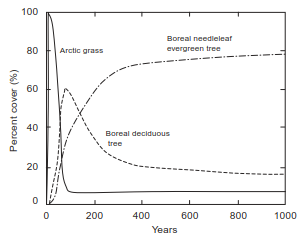
Fig. 24.23. Boreal forest stand dynamics simulated by a dynamic global vegetation model. The simulation is from initially bare ground for a single model grid cell in the boreal forest over 1000 years in the absence of disturbance. Percentage cover is the annual extent of plant functional types in the grid cell. Adapted from Bonan et al. (2003).

Dynamic Global Vegetation Models and Earth System Feedback. To overcome the computational limitations of individual-based models, scientists developed dynamic global vegetation models (DGVMs) (Prentice et al. 2007). DGVMs simulate community composition, biomass, productivity, and nutrient cycling on a global scale. Because these models are executed globally, they do not track individual species. Instead, they group species into plant functional types (PFTs), which are differentiated by attributes such as woody vs. herbaceous biomass, broadleaf vs. needleleaf leaf form, and evergreen vs. deciduous leaf longevity.

· Cohort-Based Scaling and Grid Dynamics

· Succession Simulation in Alaskan Boreal Forests

· Coupling DGVMs with Earth System Climate Models

Cohort-Based Scaling and Grid Dynamics. DGVMs do not recognize individual plants in the manner of gap models. Instead, they represent cohorts of individuals sharing similar size distributions, or represent an average individual plant alongside total population density within a grid cell. A prominent example of a DGVM is the Lund-Potsdam-Jena (LPJ) model (Sitch et al. 2003). The LPJ model characterizes vegetation as patches of plant functional types within a grid cell. Each PFT is represented by an average individual defined by mean biomass, crown area, height, and stem diameter, combined with total individual count and fractional ground cover. Vegetation structure updates dynamically in response to resource competition, allocation, mortality, biomass turnover, litterfall, establishment, and fire disturbance.

Succession Simulation in Alaskan Boreal Forests. Bonan et al. (2003) integrated the ecological principles of the LPJ model into a dynamic global vegetation model designed for coupling with global climate models (as shown in Fig. 25.13). The modeled tree biogeography aligns closely with satellite observations of tree cover and natural vegetation distributions. The model successfully reproduces primary forest succession, as demonstrated in simulations of the Alaskan boreal forest over a 1000-year period (as shown in Fig. 24.23). In these simulations:

· 1st stage: Grasses initially dominate the bare landscape.

· 2nd stage: Grass cover rapidly declines while deciduous trees increase, reaching peak abundance in under 100 years.

· 3rd stage: Deciduous cover declines as evergreen trees establish dominance.

· 4th stage: Transition from deciduous to evergreen dominance occurs around year 145, after which evergreen cover increases to 76% while deciduous trees decrease to 15%.

This simulated succession sequence closely mirrors observed field succession in interior Alaska (as shown in Fig. 22.10b). In natural settings, recurring fires prevent stands from aging beyond 250 years in this region. Simulated net primary production at year 250 (386 g C m⁻² yr⁻¹) and total vegetation biomass are highly comparable to observed values in Alaskan boreal forests.

Coupling DGVMs with Earth System Climate Models. Many biogeochemical models and dynamic global vegetation models have been developed specifically to quantify ecosystem-climate feedbacks. Designed as fully integrated components of global climate models, they link biogeophysical, hydrologic, physiological, and biogeochemical processes to construct mechanistic representations of surface energy fluxes, photosynthesis, respiration, allocation, and carbon-nutrient cycling (as shown in Fig. 25.2). Leaf phenology models the precise timing of budburst, senescence, and leaf abscission in response to temperature and drought triggers. Vegetation dynamics are driven by net primary production, mortality rates, fire regimes, and plant responses to physical disturbances.

Model structures differ significantly in how they compute environmental parameters (such as soil water and soil temperature), how these conditions affect physiological processes, and how multiple resource limitations jointly constrain net primary production and carbon allocation. Some models prioritize physical environmental controls (e.g., light absorption, soil moisture, soil thermal regimes), whereas others emphasize biogeochemical controls like nutrient availability. Furthermore, plant migration represents a major challenge in global modeling, as most current models restrict seed dispersal and range shifts based strictly on bioclimatic constraints (Van Minnen et al. 2000; Higgins and Harte 2006).

Consequently, simulated carbon uptake and storage vary considerably across model implementations. Resolving discrepancies among global ecosystem models requires improved synthesis of observational datasets, including net primary production (Scurlock and Olson 2002), leaf area index (Asner et al. 2003), vegetation carbon (as shown in Fig. 24.9a), canopy height (as shown in Fig. 24.9b), soil carbon (as shown in Fig. 24.11), and carbon and energy fluxes (as shown in Fig. 24.7). Furthermore, ecosystem models must undergo rigorous testing against comprehensive multi-source observational benchmarks across diverse spatial and temporal scales (Randerson et al. 2009; Luo et al. 2012).