Land Surface Model Evaluation and Coupled Climate Simulation

Evaluation Protocols Across Scales. Model evaluation is an essential phase in testing and validating the physiological, biogeochemical, and hydrometeorological processes simulated by land surface models across leaf, canopy, regional, and global scales. Simulated leaf-level processes—such as leaf photosynthesis and stomatal conductance—are directly evaluated against empirical field measurements. A representative study by Dang et al. (1998) evaluated a leaf photosynthesis-conductance model using empirical branch data collected from black spruce and jack pine trees across three distinct field campaigns over the growing season. Modeled leaf-scale photosynthesis demonstrated strong agreement with observations across photosynthetically active radiation levels from 0 to 1450 µmol m⁻² s⁻¹, leaf temperatures ranging from -5 °C to 35 °C, and atmospheric CO₂ concentrations spanning 50 to 900 ppm (as shown in Fig. 25.4). Modeled stomatal conductance exhibited a similarly close match to field observations (as shown in Fig. 25.4).

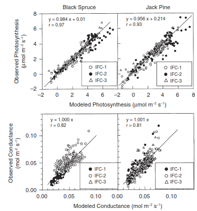
Fig. 25.4. Comparison between modeled and measured photosynthesis (top) and stomatal conductance (bottom) for branch samples of black spruce and jack pine trees. Data were collected during three intensive field campaigns (IFCs). Model parameters were derived for each IFC. Adapted from Dang et al. (1998).

Eddy Covariance Tower Measurements. Canopy-scale flux evaluation relies on high-frequency observations collected at eddy covariance flux towers. During the early 1990s, flux observations were restricted to brief field campaigns lasting a few weeks or less. For instance, Bonan et al. (1997) evaluated simulated net radiation, sensible heat, latent heat, and CO₂ fluxes against summer 1994 observations gathered at a jack pine forest site during the Boreal Ecosystem Atmosphere Study (BOREAS) (as shown in Fig. 25.5). In this study, the land surface model was run uncoupled from an atmospheric model, driven offline with observed local meteorological forcing. Averaged over a 23-day period (July 19 to August 10, 1994), the offline land surface model successfully reproduced the average diurnal cycles of surface energy components and CO₂ flux (as shown in Fig. 25.5). The principal divergence occurred during midday, when the model failed to capture the observed depression in latent heat flux (as shown in Fig. 25.5).

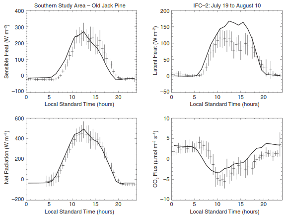
Fig. 25.5. Comparison between modeled and measured sensible heat flux, latent heat flux, net radiation, and CO₂ flux for a jack pine stand during IFC-2 (July 19–August 10, 1994) of the Boreal Ecosystem Atmosphere Study (BOREAS). See Figure 12.7 for additional information. Shown is the average diurnal cycle. Crosses show observed fluxes ± 2 standard error of the mean. The solid line is the average modeled fluxes. Reproduced from Bonan et al. (1997).

Iterative Evolution of the Community Land Model. The progressive development of the Community Land Model (CLM)—from CLM version 3 (Dickinson et al. 2006), through version 3.5 (Lawrence et al. 2007), to version 4 (Lawrence et al. 2011, 2012)—illustrates the systematic application of flux tower datasets in model benchmarking.

· Amazonian Rainforest Evaluations: Hourly evaluations of CLM3 against ABRACOS flux tower observations (April 4–July 26, 1993) in southwestern Amazonia revealed substantial biases (as shown in Fig. 25.6). CLM3 systematically overestimated sensible heat flux (r² = 0.72, slope = 2.57, RMSE = 122.00 W m⁻², bias = 63.07 W m⁻²) and underestimated latent heat flux (r² = 0.75, slope = 0.57, RMSE = 91.19 W m⁻², bias = -46.92 W m⁻²). Revised latent heat flux parameterizations in CLM3.5 significantly reduced these discrepancies, improving performance statistics for latent heat flux (r² = 0.94, slope = 1.01, RMSE = 37.13 W m⁻², bias = -8.38 W m⁻²) and sensible heat flux (r² = 0.59, slope = 1.35, RMSE = 61.06 W m⁻², bias = 26.77 W m⁻²)(as shown in Fig. 25.6).

· Temperate Forest Moisture Dynamics: Multi-year flux network observations have become standard for guiding model parameterizations (Randerson et al. 2009; Blyth et al. 2011; Lawrence et al. 2011; Wang et al. 2011; Bonan et al. 2011, 2012). Simulations at Morgan Monroe State Forest, Indiana (2003) showed that CLM3 underestimated soil moisture relative to saturation at 30 cm depth, leading to excessively low latent heat flux and high sensible heat flux during summer (as shown in Fig. 25.7). Refinements in CLM3.5 governing infiltration, runoff, soil evaporation, and groundwater dynamics resulted in wetter soils, higher latent heat fluxes, and lower sensible heat fluxes that aligned closely with empirical measurements across temperate, Mediterranean, tropical, boreal, and subalpine flux tower sites (Stöckli et al. 2008)(as shown in Fig. 25.7).

· Global Upscaled Flux Benchmark: Synthesis of individual flux tower measurements into upscaled global flux products (Jung et al. 2011) enables comprehensive benchmark testing of land models at global scales.

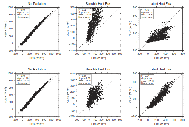
Fig. 25.6. Comparison of hourly observed (OBS) and simulated (CLM3) net radiation, sensible heat flux, and latent heat flux for tropical rainforest in southwestern Amazonia for the period April 4–July 26, 1993. Observed fluxes are from the Anglo-Brazilian Amazonian Climate Observation Study (ABRACOS). See Figure 12.5 for additional information. Modeled fluxes are for the Community Land Model version 3 (top) and a modified version of the model (bottom). Data provided courtesy of Keith Oleson and David Lawrence (National Center for Atmospheric Research, Boulder, Colorado).

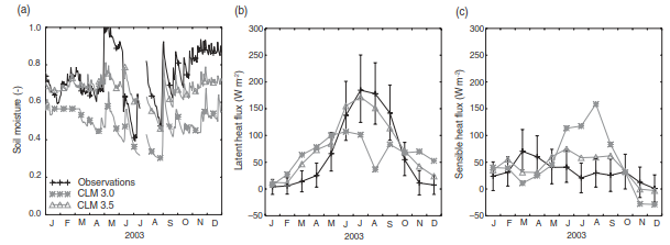
Fig. 25.7. Model simulations (gray lines) compared with observations (black lines) for Morgan Monroe State Forest, Indiana, during 2003. Shown are (a) soil moisture relative to saturation at 30 cm depth, (b) monthly latent heat flux, and (c) monthly sensible heat flux. Error bars show estimated uncertainties of observed fluxes. The gray lines show simulations using version 3.0 and version 3.5 of the Community Land Model. Adapted from Stöckli et al. (2008).

Large-Scale Hydrologic and Basin-Level Validation. Terrestrial hydrologic evaluation spans local catchments to global river basins. Monthly terrestrial water storage anomalies derived from the Gravity Recovery and Climate Experiment (GRACE) satellite mission provide critical basin-scale hydrological metrics (Lawrence et al. 2012)(as shown in Fig. 25.8). Coupled climate simulations using CCSM3/CLM3 produced muted seasonal water storage amplitudes in the Amazon basin and Mississippi basin, whereas CCSM4/CLM4 accurately captured the observed annual water storage cycles (as shown in Fig. 25.8).

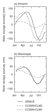
Fig. 25.8. Monthly soil water storage from GRACE and from simulations with version 3 and version 4 of the Community Land Model for (a) the Amazon basin and (b) the Mississippi basin. Adapted from Lawrence et al. (2012).

River Flow and Macro-Scale Watershed Dynamics. River flow integrates large-scale hydrological cycling across regional catchments. Comparisons between observed annual river flow and CLM simulations across the 50 largest global rivers demonstrate that the model reproduces the overall magnitude and variance of river discharge (as shown in Fig. 25.9). Local deviations in simulated river discharge stem primarily from atmospheric model precipitation biases or errors in partitioning net precipitation between evapotranspiration and runoff.

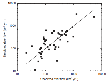
Fig. 25.9. Observed annual river flow for the 50 largest rivers and simulated annual river flow. The solid line shows the 1:1 relationship. Data provided courtesy of Keith Oleson (National Center for Atmospheric Research, Boulder, Colorado).

Catchment-Scale Model Intercomparisons. Single-site and basin-scale offline experiments demonstrate structural sensitivities across model formulations.

· Project for Intercomparison of Land-Surface Parameterization Schemes (PILPS): Standardized offline forcing experiments (Henderson-Sellers et al. 1996) revealed substantial divergences in predicted surface energy fluxes and hydrologic cycles despite identical meteorological drivers, vegetation parameters, and soil textures. Initial synthetic forcing tests over tropical rainforests and grasslands (Pitman et al. 1999) highlighted major differences in net radiation partitioning (sensible vs. latent heat) and evapotranspiration-runoff partitioning. Interactions between evapotranspiration and runoff dictate maximum attainable soil moisture (Koster and Milly 1997).

· Site-Specific Benchmark Evaluations: Offline evaluation at the Cabauw grassland site in the Netherlands underscored the influence of stomatal resistance formulations and soil moisture stress on annual flux partitioning (Chen et al. 1997; Qu et al. 1998). Data from the HAPEX-MOBILHY campaign in southern France showed large model variations in simulated soil moisture, runoff, and soil evaporation parameterizations (Shao and Henderson-Sellers 1996a,b; Desborough et al. 1996). Simulations at Valdai, Russia, demonstrated that incorporating soil water phase change energetics prevents extreme soil overcooling during winter freezing, whereas models omitting freeze-thaw phase transitions produced unrealistically cold soil temperatures (Schlosser et al. 2000; Slater et al. 2001; Luo et al. 2003).

· Macroscale Basin Watershed Studies: Catchment-scale evaluations confirm that land surface schemes reproduce large-scale energy balance and discharge dynamics across diverse river systems, including the 566,000 km² Red-Arkansas River basin (Liang et al. 1998; Lohmann et al. 1998; Wood et al. 1998), the 58,000 km² Torne-Kalix River system (Bowling et al. 2003a,b; Nijssen et al. 2003), and the 86,000 km² Rhône River basin (Boone et al. 2004).

Regional Climatology and Earth System Coupling. Regional surface climatology simulated by climate models is directly benchmarked against multi-variable observations. Multi-model comparisons over eastern Canada (latitudes 50° N to 60° N, longitudes 80° W to 55° W) across five climate model configurations (CCM3/CLM2_T42, CCSM2.0_T42, CCSM3.0_T42, CAM3/CLM3_T85, and CCSM3.0_T85) demonstrate general agreement with observed monthly 2-m air temperature, precipitation, runoff, and snow depth cycles (Dickinson et al. 2006)(as shown in Fig. 25.10).

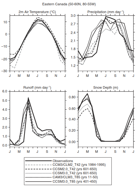
Fig. 25.10. Monthly averaged 2-m air temperature, precipitation, runoff, and snow depth compared with observations for a region of eastern Canada defined by latitudes 50° N to 60° N and longitudes 80° W to 55° W. Data are shown for five climate models that differ in spatial resolution and model physics. Reproduced from Dickinson et al. (2006).

Despite baseline agreement, structural differences among first-generation, second-generation, and third-generation land surface models remain significant (Henderson-Sellers et al. 2003; Pitman 2003). Controlled intercomparisons across seven land models revealed large discrepancies in temperature and evapotranspiration responses to imposed land-cover change (Pitman et al. 2009; Boisier et al. 2012; de Noblet-Ducoudré et al. 2012). Expanded 15-model comparisons confirmed persistent divergences in land-use sensitivity (Kumar et al. 2013) and fundamental hydrologic cycle representations (Dirmeyer 2011; Wei et al. 2010).

Coupled Land-Atmosphere Dynamics. In a fully coupled climate model, bidirectional feedback loops operate continuously between the atmospheric model and the land surface model (as shown in Fig. 25.11).

· Atmosphere-to-Land Forcing: The atmospheric model supplies temperature (T), zonal and meridional wind components (u, v), specific humidity (q), precipitation (P), downwelling solar radiation (S↓), and downwelling longwave radiation (L↓) to the land surface model at coupling intervals typically short (Δt ≤ 30 minutes)(as shown in Fig. 25.11).

· Land-to-Atmosphere Feedback: The land surface model returns diagnostic boundary fluxes, including latent heat (λE), sensible heat (H), surface momentum stress (τₓ, τᵧ), reflected shortwave radiation (S↑), and emitted longwave radiation (L↑)(as shown in Fig. 25.11).

· Experimental Vegetation Protocols: Paired climate model integrations evaluate land-cover alterations by comparing a control simulation forced with a baseline vegetation map against an experimental simulation forced with an altered vegetation map over multi-decadal time horizons (e.g., 20-year climate integration)(as shown in Fig. 25.11). The climate impact of altered vegetation cover is isolated by subtracting control output fields from experimental output fields (Experiment - Control)(as shown in Fig. 25.11).

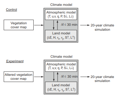
Fig. 25.11. Paired climate model simulations to examine the influence of altered vegetation cover on climate. The atmosphere model provides temperature (T), wind (u, v), humidity (q), precipitation (P), solar radiation (S↓), and longwave radiation (L↓) to the land model. The land model returns the surface fluxes of latent heat (λE), sensible heat (H), momentum (τₓ, τᵧ), reflected solar radiation (S↑), and emitted longwave radiation (L↑). The coupled land–atmosphere model is integrated for many model years with a time step typically less than 30 minutes. The climate effect of altered vegetation cover is the difference between the experiment climate and the control climate (experiment - control).