
Spatial Heterogeneity of Precipitation and Soil Moisture in Runoff Generation
The total runoff from a catchment is an integration of a number of runoff generation processes within the watershed. One such factor is the rate of precipitation, which can vary spatially depending on storm characteristics. Figure 11.6 shows the spatial distribution of rainfall over the 154 km2 Walnut Gulch watershed in Arizona during two storms. Both storms delivered a similar amount of rainfall, but they differed greatly in their spatial characteristics. The storm on September 8, 1970 was locally concentrated. The average precipitation across the watershed was 6.4 mm, but this rain fell over only 68.5 percent of the watershed with a local precipitation maximum of 39 mm. Ten percent of the watershed received more than 25 mm of rainfall. In contrast, the storm on August 25, 1972 was more evenly distributed. The spatial average precipitation was 7.3 mm. This rain fell over the entire basin. Ninety percent of the watershed received between 3 and 10 mm of rain. None of the watershed received more than 14 mm of rainfall.
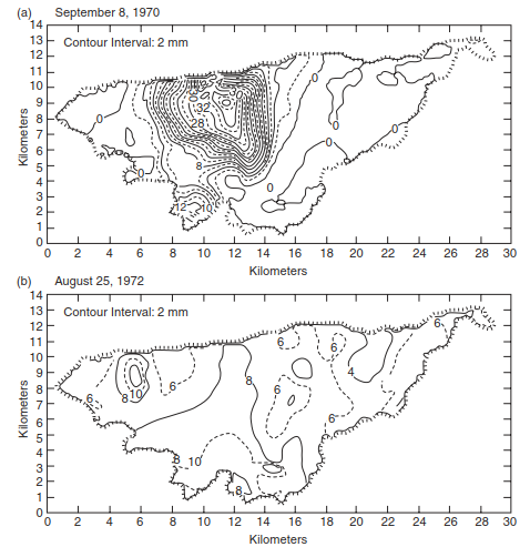
Fig. 11.6. Rainfall distribution across the 154 km2 Walnut gulch watershed near tucson, arizona, for (a) September 8,1970 and (b) august 25, 1972. Redrawn from Fennessey et al. (1986)
In addition, soil water varies spatially depending on soil texture. Figure 11.7 shows soil water content for the Little Washita watershed near Chickasha, Oklahoma. This watershed drains an area of 610 km2 and is covered by pasture rangeland and crops. Heavy rain fell across the watershed on June 5 followed by moderate rainfall until June 9. Thereafter there was no rain for several days. On June 10 volumetric soil water content in the first 5 cm of soil ranged from 0.15 to 0.35 m3 m-3. The near-surface soil was close to saturation in the west and east, where the soil is primarily silt loam and loam. Central areas, where the soil is sandy loam and sand, were drier. This general spatial pattern was maintained as the soil drained over the next few days.
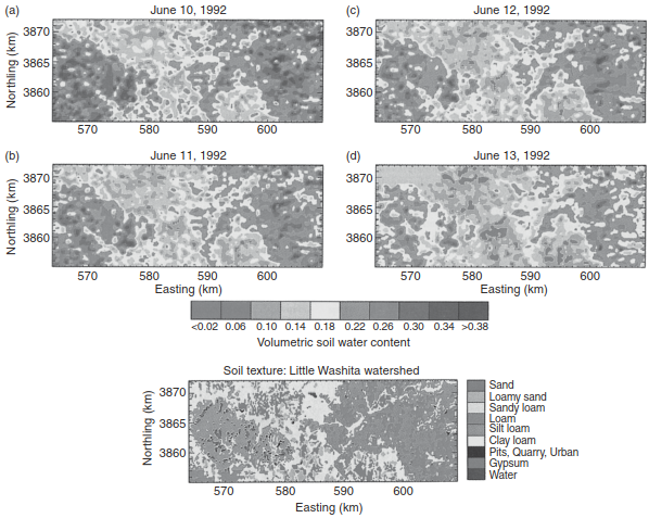
Fig. 11.7. Near-surface (0–5 cm depth) volumetric soil water content for June 10–13, 1992 in the little Washita watershed, oklahoma. data have a spatial resolution of 200 m. reproduced from mattikalli et al. (1998). See color plate section
Exponentially Distributed Precipitation. The example shown in Table 11.2 illustrates how spatial variation in precipitation affects runoff. In this particular example, the average precipitation is 1.85 mm, but the actual amount received varies with four sub-catchments. For example, 25 percent of the watershed receives only 0.2 mm of rainfall; 10 percent receives 7 mm. The total runoff from the watershed is found by applying Eq. (11.2) to each sub-area, weighted by the appropriate fractional area. In this example, 0.65 mm of runoff is generated by the watershed assuming a spatially invariant infiltration capacity of 2 mm. In contrast, no runoff is generated by the watershed if Eq. (11.2) is evaluated with the average precipitation. This is because local precipitation exceeds infiltration capacity for 40 percent of the watershed. The remaining 60 percent of the watershed generates no runoff.
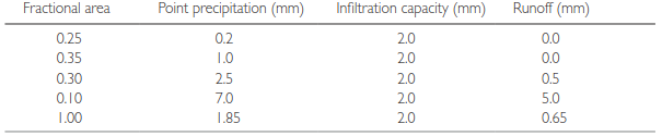
Table 11.2. Example runoff calculation for a catchment divided into four sub-areas each receiving point precipitation (P) and generating runoff (R) as the precipitation in excess of infiltration capacity (i)
One approach commonly used to account for spatial variability in precipitation is to represent the precipitation rate at a point as an exponential probability density function (Shuttleworth 1988; Pitman et al. 1990; Dolman and Gregory 1992; Eltahir and Bras 1993). Rain is assumed to fall over a fraction of the surface (µ) and the remainder (1 - µ) receives no rainfall. Within the raining area, the local precipitation rate at a given point in space (P) is exponentially distributed with the probability density function:

where P is the precipitation rate averaged over the entire surface. The average precipitation rate over the raining area is P / µ, and the rain covered portion of the surface receives higher precipitation rates as rainfall is concentrated into a smaller area (i.e., µ decreases). This is evident from the cumulative probability distribution, which gives the probability that local precipitation is less than a particular value. As shown in Figure 11.8a, the occurrence of extreme high local rainfall rates increases as µ decreases, resulting in an increase in the mean and median rates over the area µ that receives rainfall.
Equation (11.3) can be used to scale runoff at a particular point in the watershed to the entire catchment. If infiltration capacity is spatially invariant, the average runoff is obtained by integrating Eq. (11.2) with respect to P (which provides the runoff rate from the rain covered fraction µ) and recognizing that the fractional area 1 - µ receives no rainfall:

Figure 11.8b illustrates the behavior of Eq. (11.4). The amount of precipitation that becomes runoff (R / P) decreases as infiltration capacity increases relative to precipitation (i.e., as i / P increases). For a given i / P, the runoff ratio increases as the fractional area of precipitation (µ) decreases. That is, locally concentrated rainfall increases runoff.
Date added: 2026-09-24; views: 1;